Services on Demand
Journal
Article
 English (pdf)
 Article in xml format
 Article references
 Send this article by e-mail
Indicators
-
 Cited by SciELO
 -
 Access statistics
Related links
-
 Cited by Google
 -
 Similars in
SciELO
Similars in
SciELO -
 Similars in Google
Share

 Permalink
CT&F - Ciencia, Tecnología y Futuro
Print version ISSN 0122-5383On-line version ISSN 2382-4581
C.T.F Cienc. Tecnol. Futuro vol.4 no.1 Bucaramanga Jan./July 2010
Natalia García2, Carlos Becerra2, Yaqueline Figueredo1 and Alexandra Plata2
2Universidad Industrial de Santander, Bucaramanga, Santander, Colombia
e-mail: saulguevara@yahoo.com William.agudelo@ecopetrol.com.co
* To whom correspondence may be addressed
ABSTRACT
The seismic image of deep rock, interesting for the petroleum industry, can be distorted by the heterogeneous near-surface layers, characterized by low wave propagation velocity. The conventional methods used in counteracting this effect seem less effective in complex areas with rough topography such as those commonly found in Colombia, which are also affected by stronger tropical weathering. Characterization of the near-surface layer was conducted in this work with the purpose to investigate these relationships. Geological and geophysical methods were applied using data from a 2D seismic survey performed in the Catatumbo area of Colombia and seismic data and cutting samples analysis from a couple of 60 m depth wells (downhole surveys), drilled at rough surface locations. Wave propagation velocities were calculated by the application of tomography and refraction. Visual and laboratory assays such as granulometry and mineralogy were used in the analysis of the cutting samples. It was then possible to relate physical and lithological characteristics with properties of seismic response. Differences between the seismic response and the geological description were also observed and some uncertainties were identified.
Keywords: Seismic methods, static corrections, weathering, soils, strata, well logs, complex geology, seismic data, 2D seismic, seismic waves, Catatumbo basin, wave velocity.
RESUMEN
El estrato somero, heterogéneo y caracterizado por la baja velocidad de propagación de las ondas sísmicas, tiene influencia adversa en la imagen de los reflectores profundos obtenida a través del método sísmico, y de interés para la industria petrolera. Los métodos tradicionalmente usados por la industria para contrarrestar este efecto parecen insuficientes en casos de zonas complejas y con topografía abrupta, como sucede con frecuencia en Colombia. Con el objeto de contribuir a entender y superar estas limitaciones, en este trabajo se caracteriza el estrato somero usando metodologías geológicas y geofísicas. Para este objeto, se utilizaron datos obtenidos en un levantamiento sísmico 2D efectuado en la cuenca del Catatumbo, y datos de dos pozos de estudio de 60 m de profundidad, en los cuales se midieron datos sísmicos directos y, además, se obtuvieron muestras de ripios, se midieron velocidades de propagación de las ondas por varios métodos sísmicos y se hicieron ensayos visuales y de laboratorio sobre los datos de ripios. De esta manera, fue posible relacionar características físicas y litológicas con propiedades de la respuesta sísmica. También se encontraron diferencias y se identifican algunas incertidumbres al respecto.
Palabras clave: métodos sísmicos, correcciones estáticas, meteorización, suelos, estratos, registros de pozo, geología compleja, datos sísmicos, sísmica 2D, ondas sísmicas, cuenca del Catatumbo, velocidad de ondas.
INTRODUCTION
The seismic method is a key technology to obtain information about the geological characteristics of the earth crust. The main technique currently applied in the petroleum industry for onshore projects deploys energy sources and sensors on the land surface. In this case seismic waves propagate slower through the more heterogeneous near surface layer with slow velocity, frequently generating distortion in the seismic image of deeper rocks. Static correction (Cox, 1999) is the name of the method used successfully in the industry to overcome such effects. However this method appears less effective when it is applied to complex geology and/ or rough topography settings, as many zones of interest for the petroleum industry in Colombia.
Static correction is based on a very simplified wave propagation model which can explain partially the limited quality of seismic data in these settings. However specific characteristics of the weathering caused by the tropical weather alter the near surface properties, which can affect the elastic wave propagation. This topic is explored in this work.
A number of technical branches have studied the near surface. In fact, the near-surface is the main subject of fields such as geotechnical engineering and agriculture (pedology), each one with its own method and scope. Soil is the name most frequently used for this layer by these technologies, even though geotechnical engineering emphasizes its mechanical properties and Agricultural studies are more focused on its biochemical characteristics. The geotechnical approach appears closer to the focus of our interest since emphasizes the mechanical properties. In the seismic method the near surface zone is mostly identified by its low velocity, such that it is known as the low velocity layer.
As mentioned before, the near-surface layer is usually less consolidated and more heterogeneous than deeper layers. Weathering together with erosion and sediment deposition contributes to set up this layer. Tropical weathering has been subject of studies, many related with engineering applications, e. g. Islam, Stuart, Risto & Vesa (2002), Chigira, & Oyama (2000), and Fookes (1997).
Chemical weathering, due to rainy and hot climate is much stronger in tropical zones, generating in principle thicker and complex residual soils (Brady & Weil, 1996; Malagón, 1995). Rocks are affected by processes like dissolution, oxidation and hydrolysis. As a result materials like ferric oxides (such as hematite) and clay minerals (like kaolinite and others) are typical products of chemical weathering (see e.g. Brady & Weil, 1996, Tarbuck & Lutgens, 2005).
From a geotechnical engineering approach, Fookes (1997) proposes for tropical areas a typical rock weathering scale of six grades, corresponding to progressively shallower horizons, as follows:
- : Fresh rock
- : Slightly weathered.
- : Moderately weathered
- : Highly weathered.
- : Completely weathered
- : Residual soil.
The grade IV, defined as "More than half of the rock material is decomposed or disintegrated to a soil" corresponds to the limit soil-rock for engineering purposes, that is to say, at which the mechanical behavior changes (Fookes, 1997).
An approach that takes advantage of the near surface layer knowledge is proposed here. Objectives of this work are contributing to obtain a more reliable model of the near surface to improve the static corrections on images of deep reflectors in tropical settings of rough topography like many places of interest for the petroleum industry.
Geophysical and geological methods are applied. These methods include measurements of propagation times in wells, macroscopic and composition analysis of cuttings extracted from these wells, and near-surface models using tomography and refraction methods on 2D seismic data. The lithological characteristics are correlated to wave propagation velocities.
The first part describes the general characteristics of the settings and the methods used. Then, the authors present the results corresponding to each analysis method and, finally, these results are analyzed to draw the pertinent conclusions.
METHODS
Geophysical and geological methods were applied to analyze near surface data in a location of NE Colombia. It was used data from a 2D seismic survey, acquired in 2005 at that location. Two downhole surveys in 60 m depth wells were performed at two of these seismic lines. Geological methods such as cuttings analysis and Geophysical methods such as refraction and tomography were applied.
Site location and geology
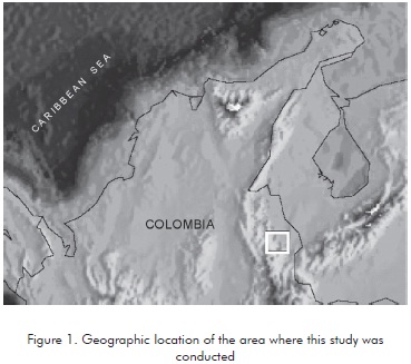
Figure 1 illustrates the location of the area where this study was conducted. Figure 2 shows the seismic lines and the shallow holes location, together with a generalized geological column in the area.
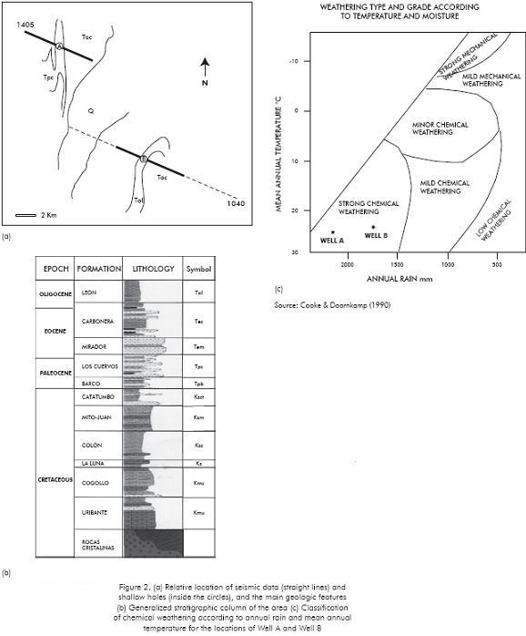
Among the geological formations, the more important for this work were León, Carbonera and Los Cuervos Formations; since they correspond roughly correspond to the location of the wells. The León Formation (Tol) is characterized by fine granulometry, showing gray and spotted arcillites, and silicon siltites, some of them with plant and organic matter debris. Small interbedding of gray mudstone with sublithic sandstone in thin layers (occasionally of medium thickness) can be observed in this formation, although they do not predominate in the whole area. Although outcrops are rare and frequently altered, the formation can be identified due to the smooth geomorphology generated. This formation has an average thickness of 545 m, and its age has been identified as Upper Oligocene - Miocene.
The Carbonera Formation (Tec) has an average thickness of 500 m, and its age has been identified as Upper Eocene to Lower Oligocene. It is composed by claystones interbedded with sandstones. Some coal layers appear in the upper and lower sections. Claystones are grayish, some of them dark and chert especially in the upper and lower sections. The sandstones are usually gray-greenish, a bit clayish and fine to coarse grained Los Cuervos Formation (Tpc) is composed of chert clay, and lime claystones interbedded with fined grained sandstones and with coal layers mostly at the lower part.
Numerous coal mines are found on this Formation. Over the carboneous section, mostly gray and graygreenish claystone are present. Hard sandstones layers are also present over all the Formation. Its bottom can be identified where the Barco Formation sandstone appears below the coal layers. The thickness span from 245 m to 490 m, with a mean about 320 m. Its age is mostly Paleocene, and its youngest part has been identified as Late Eocene.
Climate
Chemical weathering depends on the climate, mostly moisture and temperature. The relationship between mean annual temperature and annual rain, and the type of chemical weathering is shown in Figure 2c, taken from Cooke & Doornkamp (1990), Information about rain and temperature for this zone was investigated using local records, and the data about these climate indicators for the locations corresponding to Well A and Well B are also depicted in the figure. It is shown that these settings are identified as corresponding to strong chemical weathering.
Downhole Records
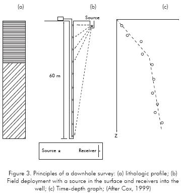
Shallow boreholes allow obtaining direct information of the near surface. According to Cox (1999), there are two configurations for shallow boreholes. The first one, known as uphole survey, is composed by several sources within the hole and one or more receptors on the surface. The second one, known as the downhole method, requires sources on the surface and receptors within the hole. It is illustrated in Figure 3. This downhole configuration was used in the experiments of this study.
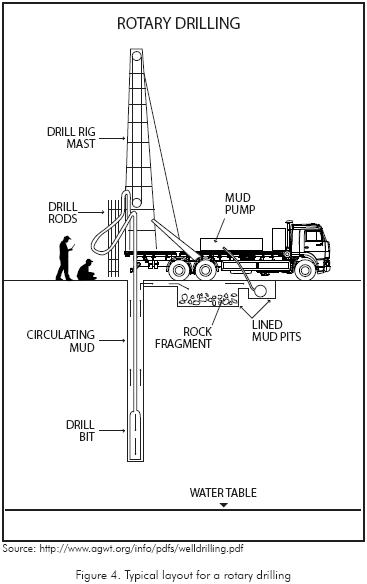
Drilling
Drilling was carried out using a rotary tricone bit provided of a derrick and mounted on a truck. Figure 4 illustrates the features of such a machine. A mud-water mixture is injected into the bit, in order to reduce the friction heat and to take out to the surface the residue rock fragments, which are deposited in a pool with this purpose. From these fragments are selected the cuttings used subsequently for analysis.
The shooting scheme is illustrated in Figure 3. The sample interval (distance between receivers) in this downhole is 5 meters, from 15 meters to 60 meters depth. The zone corresponding to the first 15 meters has more detailed sampling and, consequently, more detailed control of lithological changes.
The downhole A is located in the seismic line identified with the number 1405, in an EW direction, probably on the Los Cuervos Formation (Figure 2a). The downhole B is located on the Seismic Line 1040 (see map in Figure 2), in rocks belonging to the León Formation.
Arrival times of the seismic waves contain information about the velocity of the geological. The downhole record interpretation includes:
- Finding the peaks corresponding to the first arrivals from each receptor.
- For surface receptors, application of some necessary corrections to these times (geometric correction) (Cox, 1999).
- Drawing of graphs and calculation of the velocity and thickness corresponding to the identified layers. (Figure 3).
A methodology proposed by Rueda (2009) was used as a first approach to interpret the geologic layering in terms of the velocity variation. After that, geological criteria defined the model selected.
Cuttings, together with cores, provide direct information about the subsoil and shallow geology. In this study, the well drilling generated cuttings which were subject of the geological analysis methods.
Macroscopic (shape, size, and distribution) as well as compositional analysis of the cuttings were carried out, using magnifying glass, sieving and acid reaction test to identify differences between the weathered layer and the fresh rock. A mineralogical composition analysis was carried out with the aid of laboratory methods such as X-ray diffraction with the purpose to identify typical weathering products such as kaolinite and goethite. These analyses can also contribute to identify parental rocks if present.
Indirect methods: refraction and tomography
From seismic data collected on the surface, indirect methods yield information about the shallow subsurface. There are seismic events travelling through the near-surface, which provide information about this zone. Refraction methods have traditionally been used to determine a near-surface velocity model, to be used for the statics correction process. These methods assume that the first arrivals basically correspond to refracted waves traveling through layers close to the surface. Many methods for analyzing refraction data have been developed (e.g. Cox, 1999). A model of the near-surface layer using the Generalized Reciprocal method (GRM) was applied here. Its principles are presented in the Appendix A.
More recently, seismic tomography has been applied to obtain velocity models developed for inversion of seismic refraction data. Instead of the layered model assumed by the refraction method, tomography requires to define a grid, allowing a different velocity for each grid element, hence a more irregular geometry in the model. Both methods assume an isotropic elastic medium.
Tomography was also applied to the data of this study, using a well established method applied in the industry. The principles of this method are summarized in Appendix B.
RESULTS
Downhole and cuttings analysis
Downhole A
Figure 5 illustrates the seismic wave arrival times in this well. Figure 5a shows the field data and Figure 5b the first arrivals picking. A three-layer structure can be identified from these arrival times. The first one has a velocity of 940 m/s and reaches 6 m depth, the second one has a velocity of 4180 m/s and spans from 6 m to 28 m depth, and the third one has a velocity of 2830 m/s and goes to the bottom of the well.
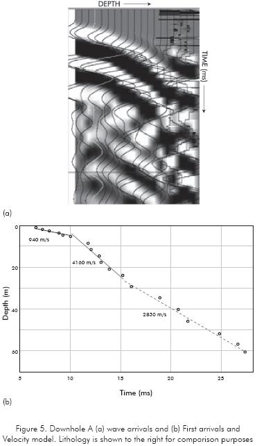
Figure 6 illustrates the data resulting from the geological analysis. Figure 6a shows a qualitative model resulting of the macroscopic and compositional analysis of the samples, and Figure 6b shows the percentage for each one of the materials identified.
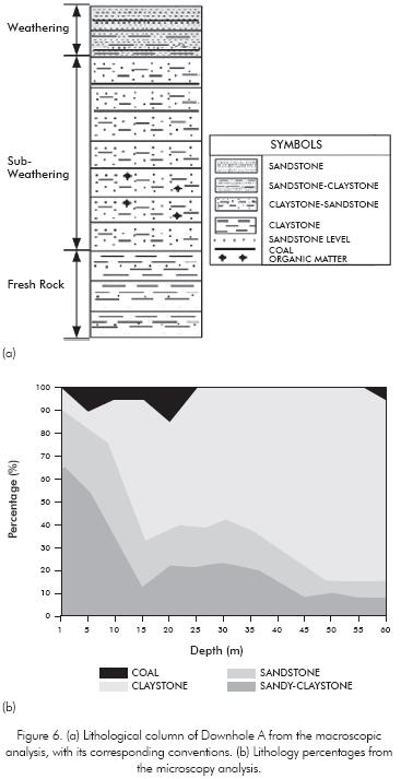
Red and yellow material dominates in the first 5 meters, exhibiting low compaction and low reaction with hydrochloric acid. It is identified with sandy-claystone in Figure 6. The percentage of this reddish material is greater in the shallower part (63% of the total sample) and decreases to 38% at 5 meter depth and to a range between 17% and 35% below 10 meters depth. Prevalence of parental rock, composed mostly by clay, can be identified below 10 meters depth. However it was more clearly interpreted as fresh rock below 45 meters depth (Figure 6a). Coal samples include about 10% of the volume over 25 m depth. The color of the shallower meters suggests a chemical-type weathering that might be caused by water related alterations.
In the macroscopic description, claystones are the most common material, followed by sandstones. Sandstone impregnated with bitumen was found in the first 30 meters, with the impregnation percentage decreasing as it becomes deeper. The dominant lithology below that level consists of clay-like rocks with the presence of a small amount of organic matter. The deeper dominant lithology corresponds to competent sandstones layers interbedded with shale, decreasing this shale content toward the bottom of the well.
From X-ray diffraction, secondary minerals found were pyrite, calcite, goethite, and rock fragments such as shale and organic matter in some cases. Quartz represents a large proportion throughout the well. The main clay mineral found was Kaolinite. However, a more quantive analysis was not possible, which can be related to the sampling procedure used.
Correlating lithology with the velocity model can be tried. The first velocity layer (940 m/s) can be identified as the most weathered layer. The second velocity layer of 4180 m/s coincides with the position and thickness of coal mantles (Figure 6a) which is consistent with the description of the Los Cuervos Formation (Ingeominas, 1967). However there is no clear explanation for this high velocity, since from the literature the P-wave velocities for coal is frequently lower (e.g. Greenhalgh, Suprajitno & King, 1986), excepted by the presence of hard coal like anthracite. A relation with the near-surface hard layers known as duricrust (Fookes, 1997) could explain this property. Finally the third layer identified at 28 m depth and below has a velocity that corresponds to the fresh rock; however it doesn't looks like that according to the macroscopic analysis (Figure 6a).
Downhole B
The data obtained from the Well B is presented in Figure 7 and 8. Figure 7 shows the first breaks analysis, which allows identifying four layers. The first layer has a thickness of 4,8 m and a velocity of 850 m/s, the velocity of the second layer is 2140 m/s and its depth goes to 18 m, the velocity of the third layer is 2000 m/s and its deep goes to 40 m and the fourth layer goes to the bottom of the well (60 m) with a velocity of 2820 m/s..
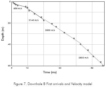
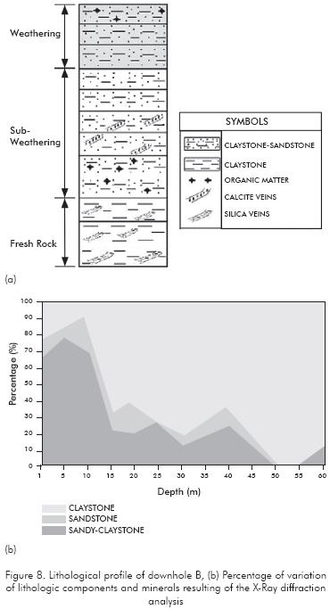
Figure 8a and Figure 8b illustrate the lithological profile corresponding to downhole B. The first layer has a thickness of 5 m, with organic matter present. The second layer is thin and could serve as a marker horizon for other analyses. Its depth ranges between 5 and 10 m. Compared to the other layers, the sandstone content in this sector is much greater and sandy red claystones predominate here.
The best defined layer is the third one, with a depth of 10 to 28 m. which has no organic matter and a high content of gray arcillites (60%), with lower content of sandy red claystones The fourth layer has a depth of 28 to 39 m and a it is possible to observe the presence of calcite veins in gray arcillites. The last part of the profile includes the presence of organic matter at the 40-50 m interval and is mostly composed by claystone. From the visual analysis weathering, subweathering and fresh rock were also separated (Figure 8a).
A correlation between the well time data and the lithologic profiles could also be attempted here according to Figures 7 and 8. In Figure 8b, characteristics about the type of lithology can be identified based on the analysis that reddish and orange colors correspond to oxidized clay-sand components with a higher degree of weathering, compared to the lighter color associated with the not oxidized material. According to this criteria, strong weathering effect can be observed shallower than 15 m depth and a weaker weathering could be identified between 15 m up to 45 m. However low velocity only reaches a depth of 5 m and after that the velocity is about constant to 40 m. This disagreement could be related to the water table level. On the other hand, the deeper part shows a good agreement between high the velocity and the rock interpreted as fresh.
Indirect methods
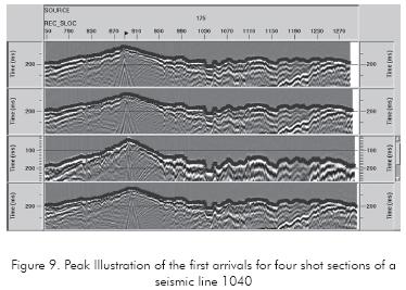
From seismic data collected on the surface, indirect methods yield information about the shallow subsurface. In this case, the first arrival times containing information about the near - surface layer were used, either according to refraction or tomography models. Figure 9 illustrates some shot records from seismic reflection line 1040 (Figure 2), with the first arrivals highlighted in red. These data, are the basis for the analyses presented in the following, based on the GRM method (Palmer, 1980) and seismic tomography.
Seismic refraction
Seismic refraction has been the method traditionally used to obtain velocity models of the near-surface layer for statics corrections. It assumes that the first arrivals basically correspond to refracted waves traveling through the interfaces closest to the surface. Therefore, these waves allow information to be obtained from the corresponding layers. It is important to note that many methods for analyzing refraction data have been developed (i.e. Cox, 1999)
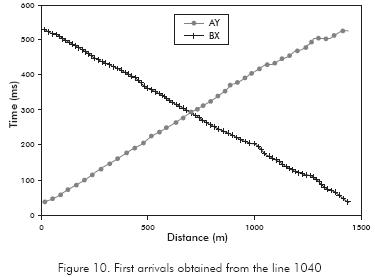
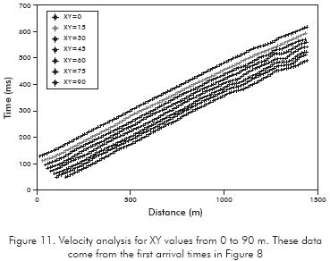
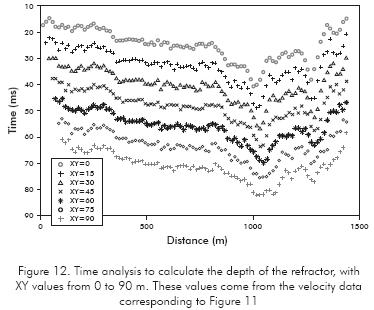
A model of the near-surface layer using the GRM method was completed. The principles of this method are presented in the Appendix A. With the information of the first arrivals obtained from the seismic line (Figure 10), the velocity-times (Equation A1) shown in Figure 11 were obtained. Based on these, the lateral variation of velocity in the refractor was calculated, using the XY separation of 15 m as the optimum value (Palmer, 1980). It can be noted that there are three lines with the following distance values: from 0 to 450 m; from 450 to 1035 m, and from 1035 to 1440 m with the corresponding velocity values of 2756, 2786 and 3231 m/s. The next step was to calculate the time values corresponding to depth (Equation A2), (Figure 12), using the information obtained from Figure 11. In this figure, the value of XY = 15 m defines best the refractor surface. This information allowed us to find a model of the velocity of the near-surface layer and the depth of the refractor. Finally, the nearsurface layer model of Figure 13 was obtained. The low-velocity layer corresponds to 831 m/s, with an average thickness of 26 m. The refractor has several lateral variations in velocities corresponding to 2756 m/s in a 450 m distance, a velocity value of 2786 m/s from 450 to 1035 m in the León Formation and a velocity value of 3231 m/s from 1035 to 1440 m in the Carbonera Formation.
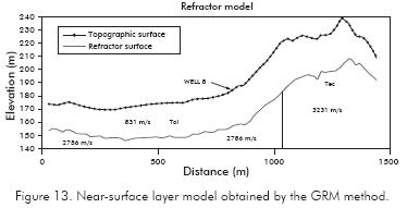
Therefore, it can be observed that the horizontal variation of velocities corresponds to the geological characteristics. Thickness, however, does not correspond to the well data.
Tomography
The tomography inversion technique (e. g. Lo & Inderwiesen, 1994) have been applied to obtain a velocity model for the near-surface layer. Since the use of these techniques discretize the medium in 11x11 m grids, several average velocity and thickness values have been used. As a result of the inversion iterative process, a 2D tomography model has been obtained.
This model, illustrated in Figure 14, does not assume strata but gradients of any geometric shape.
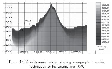
It is important to highlight the capacity of this method to reconstruct lateral variations of velocity due to lithologic changes along the line. This verifies the geologic information from cartographic descriptions of the zone and represents a significant advantage in the characterization of the near-surface layer in complex geology zones with rough topography.
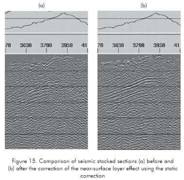
To illustrate the effect in the seismic section of the correction of the near-surface layer effect, it is shown in Figure 15, a comparison of line-B stacked section before (Figure 15a) and after (Figure 15b) the static correction, based on the refraction model.
DISCUSSION
Using information from different sources, such as seismic data, well data, and field geology can contribute to obtain a more reliable velocity model and, therefore, to correct the near-surface layer effect in the exploration seismic data.
Well information is in principle more reliable than seismic data. From Figure 6 lithology from direct measurements in well A is consistent with the description of the Cuervos Formation (Ingeominas, 1967), however there are meaningful differences with the model resulting of first breaks. According to Figure 5 three-layer model is suggested, including a shallow layer which includes a high velocity layer between 6 and 25 m. Not too much clues about this layer are found in the cuttings analysis unless the coal presence at the same depth. Weathering can be identified by the oxidized material closer to the surface in cuttings, which reach to 15 m. However the first layer according to the velocities observed correspond to 6 m. The velocities of the bottom of the well, which can be identified with fresh rock, appear at 28 m depth and downward. The sub-weathering was identified as reaching 45 m depth, according to the cuttings visual analysis.
A similar landscape can be noted in Well B, however without the high velocity anomaly closer to the surface of Well A and with a fresh rock that appears at a depth corresponding to the observed for the bottom of the subweathering. The lower velocity does not correspond to any clearly observed event in the cuttings, and oxidized material reach deeper than this lower velocity layer.
Information about the near surface was obtained using refraction and tomography methods on Line 1040, which crosses over the location of Well B. The result of the GRM method shows some correlation with the well velocities. The low-velocity layer corresponds to 831 m/s, with an average thickness of 26 m. The refractor has several lateral variations in velocities corresponding to 2756 m/s in a 450 m distance, a velocity value of 2786 m/s from 450 to 1035 m in the León Formation and a velocity value of 3231 m/s from 1035 to 1440 m in the Carbonera Formation. Therefore, the horizontal variation of velocities corresponds to the geological characteristics. Thickness, however, does not correspond to the well data with that velocity, which is about 6 m. The GRM method (Figure 13) also shows horizontal velocity variation with higher velocity in the hill, as would be expected for the corresponding hard rocks. It would means agreement between geology and GRM method.
The tomography results show a better correlation with the expected results regarding thickness and velocity values, particularly in the mountainous zone. Apparently, this is more consistent with geology than the refraction result. However important difference remains. An explanation can be related to the lower resolution of the refraction methods. Possibility of polar anisotropy can also be considered to explain this result.
The relationship between velocity observed directly in the wells and the lithology identified with cuttings analysis is not direct (Figures 5, 6, 7 and 8). Velocity variations do not necessarily correlate with lithological changes and vice versa. The presence of a ground water table could be related to such a phenomenon. It can also be related to the resolution of seismic data, that is to say, to the wavelength of the seismic event. There are also experimental or sampling uncertainties, since the cuttings collect is a procedure prone to errors.
CONCLUSIONS
- It was observed that velocity values obtained from well data are related to the parental geologic formation of each corresponding site. Features of a tropical residual soil and its thickness were also identified.
- A correlation between the velocity data obtained from the well records and the results of the lithologic model from cutting and geological analysis was found, however also with important differences. The water table can be a factor that determines this difference.
- The refraction GRM method agreed with the well information about the velocity values of the rocks corresponding to the León and Carbonera formations. The horizontal velocity variation within a layer appears geologically reasonable. However the refraction result did not correspond to the thickness information of the well. This inconsistency could be related to the characteristics of the first arrivals like its frequency content (resolution) and/or to the limitations of the GRM method in complex geology (Palmer, 1980). Anisotropy (different velocities in vertical and horizontal directions) could also be present.
- The tomography results appear correlated with the expected results from the wells regarding thickness and velocity values, particularly in the mountainous zone. Apparently, even smoothed, this is more consistent with geology than the refraction result. However there are meaningful differences, similar to the case of GRM method, which can be related to the explanation of the previous point.
- If the near surface has lateral variations in physical properties, rough topography and geologic characteristics affected by tropical weathering, well data could contribute to the improvement of the velocity model. However, there are noticeable differences between the experimental data of different sources observed in this case. Complementary data, such as cores carefully taken from wells, well logs, and more extensive research about properties like anisotropy and water table, can contribute to obtain more constrained models.
ACKNOWLEDGMENTS
The authors express their gratitude to Ecopetrol's Exploration vice-presidency for providing the data, particularly to Cristina López, Horacio Acevedo and Carlos Guerrero. Also, they thank the UIS-ICP Agreement 005 of 2003, for its support to this research, to Alba Mesa and Nestor-Raúl Moreno for their guidance in the geological analysis, and to Constanza Gómez and Yazmín Pelayo for their pioneer work. Also to the anonymous reviewers for their contribution.
REFERENCES
Brady, N., & Weil, R. (1996). The nature and properties of soils. New Jersey, USA: Prentice Hall. [ Links ]
Cooke, R. U., & Doornkamp, J. C. (1990). Geomorphology in environmental management. Oxford,UK: Clarendon Press. [ Links ]
Cox, M. (1999). Static corrections of seismic reflection surveys. SEG (Society of Exploration Geophysicists). Geophysical Reference Series, Tulsa, OK, USA. [ Links ]
Chigira, M., & Oyama, T. (2000). Mechanism and effect of chemical weathering of sedimentary rocks. Engineering Geology, 55 (1), 3-14. [ Links ]
Fookes, P. (1997). Tropical residual soils. The Geological Society Publishing House, London, UK, (Typeset by Bath Typesetting, Bath, UK, Printed by The Alden Press, Osney Mead, Oxford, UK). [ Links ]
Greenhalgh, S. A., Suprajitno, M., & King, D. W. (1986). Shallow seismic reflection investigations of coal in the Sydney Basin. Geophysics, 51,1426-1437. [ Links ]
Ingeominas, (1967). Geología del cuadrángulo F-13, Tibú, Ingeominas, Bogotá, Colombia. [ Links ]
Islam, M. R., Stuart, R., Risto, A., & Vesa, P. (2002). Mineralogical changes during intense chemical weathering of sedimentary rocks in Bangladesh. J. of Asian Earth Sciences (20), 889-901. [ Links ]
Lo, T. W., & Inderwiesen, P. L. (1994). Fundamentals of seismic tomography. SEG (Society of Exploration Geophysicists). Geophysical Monograph Series, Tulsa, OK, USA. [ Links ]
Malagón, D. (1995). Suelos de Colombia. Instituto Geográfico Agustín Codazzi. Santafé de Bogotá. D.C. [ Links ]
Palmer, D. (1980). The generalized reciprocal method of seismic refraction interpretation. SEG (Society of Exploration Geophysicists), Tulsa, OK, USA. [ Links ]
Rueda S. D. (2009). Aplicación de métodos de interpretación de la refracción sísmica en la obtención de modelos del estrato somero en el area del Catatumbo y su efecto en la imagen sísmica. Tesis pregrado. Escuela de Geología, Universidad Industrial de Santander, Bucaramanga, Colombia. [ Links ]
Tarbuck, E. J. & Lutgens, F. K. (2005). Earth: an introduction to physical geology. New Jersey, USA: Prentice-Hall. [ Links ]
APPENDIX A
THE REFRACTION GENERALIZED RECIPROCAL METHOD (GRM)
This method was proponed by Palmer (1980). It requires reciprocal, forward and backward arrival times (Figure A1).
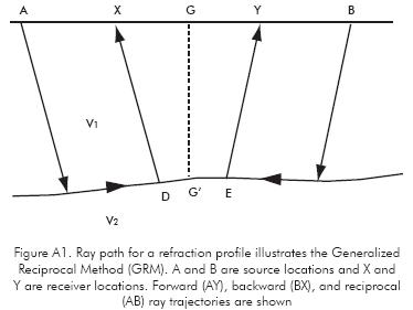
This method is accurate for dip angles below 20' and can be used in the presence of velocity gradients. It can also detect hidden layers and velocity inversions, if the refractor offset distance or displacement (horizontal distance of the ray from the refractor emergence to the receiver location) can be measured with enough accuracy.
To obtain the previous result, the value XY (distance between the receivers X and Y) should be firstly calculated, and the refractor velocity should be applied. For which it's necessary to consider the speed analysis (tv) and the time-depth widespread values (tG).
tv is defined as,
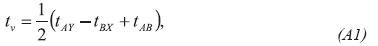
Where tAY is the transit time from the A source to the Y receiver, tBX is the transit time from the B source to the X receiver and tAB is the transit time from the A source to the B source, or the reciprocal time.
Equation A1 is applied on the localization of the G point, half way between X and Y.
The optimum XY value is given when the localizations of X and Y receivers correspond to the 2 emergent rays of a same point in the refractor, that is to say when D, G' and E coincide (Figure A1). The optimum XY value is given when the speed analysis function (tv) is the simplest among a series of speed functions (tv) derived of different values of distances among X and Y, in the refraction inverse profile, and their inclination is equal to the inverse of the apparent refractor speed.
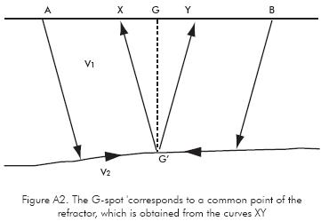
The XY value is an indicator of the refractor's depth, in other words, if the refractor is very superficial, the value of the distance among X and Y is almost zero, while, as the refractor becomes deeper the distance among X and Y receivers becomes bigger. If the distance among receivers is forced to be equal to zero (XY=0), then, the Equation 1, gives an image of the speeds in the refractor.
Once the optimum XY value and the apparent speed in the refractor for the umpteenth layer are calculated (V'n) Equation A2 may be used to derive the time-depth generalized values (tG).
tG is defined as,
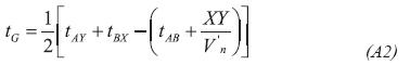
To obtain a relative image of the depths the distance XY is forced to be equal to zero (XY=0) and it's replaced in the Equation A2, being X and Y the same localization of the receiver.
APPENDIX B
SEISMIC TOMOGRAPHY
Seismic tomography allows building the velocity field of the near surface from the information obtained of the first arrival times, using inversion techniques and ray tracing theory.
Expansion series method algorithms than allow curved ray-paths are used here (Lo & Underwiesen, 1994). The medium is discretized in a number of cells of appropriate size. An initial physical model is assumed, which generates predicted data (first arrival times in this case) after applying the physical model equation (ray tracing in this case). The predicted data are referred as Ppred and the observed data are referred as Pobs in the following. An iterative procedure follows. It is carried out by comparing the observed data Pobs with the predicted data Ppred, as a function of a property of interest, which is the velocity field in this case, identified as M.
In general the relationship between the medium and the data for a discretized medium of J cells can be represented as follows:
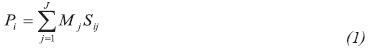
Where Pi is a vector containing transit times, Mj is a vector containing the parameter of interest of the delimited environment and Sij is a matrix with the travel path length of the i-th ray in the j-th cell.
For the real model Mtrue it is possible to obtain the observed times Pobs so that the previous expression is:

This expression can be solved as follows:


Where S-g is the inverse generalized linear operator.
This equation is usually ill-conditioned, sparse and huge sized, which makes it difficult to solve. A method to find an approximate solution is the Kaczmarz algorithm (Lo & Inderwiesen, 1994). This is an iterative method which assumes an initial model Minit, and then a calculated time vector is obtained by ray-tracing, and compared with the observed travel times. If the difference is small enough the estimated model is the solution of the problem. If not, the model should be updated according to the following equation:

Where ΔiM is the increase required to update Mest and can be represented by the following expression: