Services on Demand
Journal
Article
 English (pdf)
 Article in xml format
 Article references
 Send this article by e-mail
Indicators
-
 Cited by SciELO
 -
 Access statistics
Related links
-
 Cited by Google
 -
 Similars in
SciELO
Similars in
SciELO -
 Similars in Google
Share

 Permalink
CT&F - Ciencia, Tecnología y Futuro
Print version ISSN 0122-5383On-line version ISSN 2382-4581
C.T.F Cienc. Tecnol. Futuro vol.4 no.1 Bucaramanga Jan./July 2010
2Columbus Energy Sucursal Colombia, Cra 7 # 71-21 Ofic. 1402B, Bogotá, Colombia
3The University of Oklahoma, 100 E. Boyd St., Norman, OK, 73019, USA
e-mail: fescobar@usco.edu.co yhernandez@columbusenergy.com.co dtiab@ou.edu
(Received, Jan. 29, 2010; Accepted May 26, 2010)
* To whom correspondence may be addressed
ABSTRACT
In this work, the conventional cartesian straight-line pseudosteady-state solution and the Total Dissolved Solids (TDS) solution to estimate reservoir drainage area is applied to constant-pressure reservoirs to observe its accuracy. It was found that it performs very poorly in such systems, especially in those having rectangular shape. On the other hand, the pseudosteady-state solution of the TDS technique performs better in constant-pressure systems and may be applied only to regular square- or circular-shaped reservoirs with a resulting small deviation error. Therefore, new solutions for steady-state systems in circular, square and rectangular reservoir geometries having one or two constant-pressure boundaries are developed, compared and successfully verified with synthetic and real field cases. Automatic matching performed by commercial software sometimes are so time consuming and tedious which leads to another reason to use the proposed equations.
Palabras clave: reservoir, pressure, well testing, reservoir drainage area, pseudosteady state, TDS Technique.
RESUMEN
En este trabajo se aplica la solución convencional de análisis cartesiano para estimar el área de drenaje en yacimientos con fronteras a presión constante para verificar su exactitud. Se encontró que esta produce resultados muy pobres, especialmente en yacimientos con geometría rectangular. Por otro lado, la solución de estado pseudoestable de la técnica TDS trabaja mejor en sistemas a presión constante y se podría aplicar con un pequeño margen de error en sistemas regulares con geometría circular o cuadrada. Por tanto, se desarrollaron nuevas soluciones para sistemas en estado estable con geometría circular, cuadrada y rectangular que tienen una o más fronteras de presión constante. Estas se compararon y se probaron exitosamente en casos simulados y de campo. El ajuste automático efectuado por los paquetes comerciales algunas veces consumen mucho tiempo y son tediosos. Esto proporciona otra razón para usar las ecuaciones aquí propuestas.
Key words: yacimientos, presión, pruebas de presión, área de drenaje del yacimiento, estado pseudoestable, técnica TDS.
INTRODUCTION
The first solution for the estimation of the reservoir drainage area was presented by Ramey & Cobb (1971) from the pseudosteady-state pressure solution case. The late-time pressure data during the pseudosteady-state period behave linearly with flowing pressure and, therefore, its slope leads to the estimation of the drainage area. Later on Tiab (1994), introduced a more practical and easy-to-use solution which uses the point of intersection between the late-time pseudosteady-state period with the extrapolation of the horizontal radial flow regime straight line as part of the TDS technique, Tiab (1993). This solution works perfectly in either circular, square or rectangular closed systems, but it fails to provide accurate results constant-pressure systems having a rectangular or elongated geometry, therefore, its application as currently done so far leads to severe mistakes in the estimation of the reservoir drainage area. Another solution presented by Chacón, Djebrouni, & Tiab (2004) uses any arbitrary time and pressure derivative point read during the latetime pseudosteady state period to easily and exactly provide an estimation of reservoir drainage area in closed systems. A great advantage of this solution is the fact that it does not involve the reservoir permeability in the calculations and can be usefully used whenever the radial flow data is highly noisy. However, care should be taken in designing and running the test long enough so the latetime pseudostate/steady state period is well developed.
MATHEMATICAL BACKGROUND
The dimensionless quantities used in this work are:
The general pseudosteady-state equation was proposed by Ramey & Cobb (1971) as:
From this, the cartesian slope during the late pseudosteady- state period was defined as:
Which implies that the reservoir drainage area can be estimated from the slope of a cartesian plot of pressure versus time during late-time pseudosteady-state period.
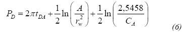
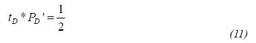
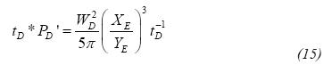
Following the philosophy of the Tiab's Direct Synthesis Technique Tiab (1994), developed an equation to estimate reservoir area using the intercept of the pressure derivative of Equation 6 with the derivative during infinite-acting radial-flow regime, (tD*PD' = 0,5):
Also, reservoir drainage area can be estimated using any arbitrary point on the pressure derivative curve during the late-time pseudosteady-state period, tpss and (t*ΔP')Pss, Chacon et al. (2004):
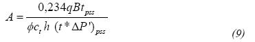
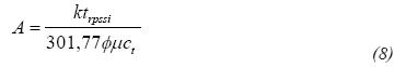
For steady-state cases, the slope of the Cartesian plot of pressure versus time may be used so Equation 7 can be applied. On the other hand, Equations 8 and 9 may also be used if a negative unit slope is drawn tangentially to the pressure derivative curve during the steady-state period; then, the intercept with this line with the straight line of the radial-flow regime or a point touched by the tangential line are, respectively, used in the mentioned equations. We should be aware that pressure and pressure derivative behaves differently for constant-pressure case systems; then, application of the above equations should lead to unaccuarate area estimations. Therefore, the following section deals with this situation in order to overcome the problem.
Square or Circular Reservoirs
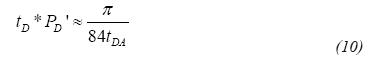
The negative unit-slope straight-line tangential to the pressure derivative curve during the steady-state period (Figure 2) is given by the following approximation:
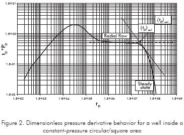
During the infinite-acting radial-flow regime, the dimensionless pressure derivative is governed by:
An equation for the drainage area is obtained from the intersection of the steady-state and the radial- flow regime lines. After plugging the dimensionless time quantity in the resulting equation will provide:
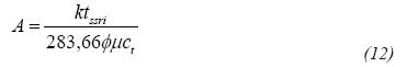
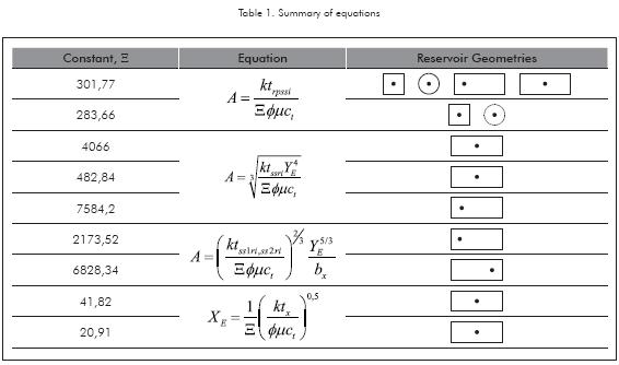
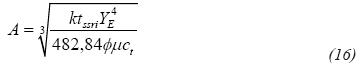
Suffix ssri stands for the intersection between the negative unit-slope line drawn tangentially to the pressure derivative curve with the radial line. It should be clarified that Equation 8 applies to any closed reservoir geometry, but Equation 12 only applies to either circular or square shape drainage area as indicated in Table 1.
Rectangular systems
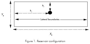
Equations 7 to 9 work well for alongated closed systems but do not apply to long reservoirs with either one or both extreme boundaries subjected to constantpressure conditions. The reservoir configuration is given in Figure 1. For such systems the governing equation depends upon several conditions:
Well centered (Figure 3)
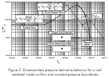
One constant-pressure boundary
Both constant-pressure boundaries
Well off-centered
Well near a constant pressure boundary - closed-far boundary (Figure 4)
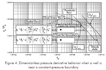
Well near a constant pressure boundary - constantpressure far boundary (Figure 4)
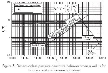
Well near a no-flow boundary - constant-pressure far boundary (Figure 5)
Well Centered
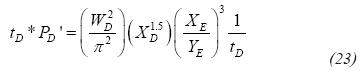
The governing equation of the negative-unit slope tangential to the pressure derivative curve for a well centered inside a rectangular reservoir with one constant-pressure boundary (Figure 3) is given here as:
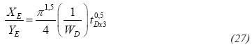
The equation for drainage area is derived from manipulation of Equations 11 and 13, assuming A=XEYE and replacing the dimensionless expressions, Equations 2 to 4, in the resulting equation, to yield:
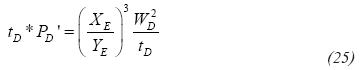
When both lateral boundaries are subjected to constant pressure, the governing equation of the negativeunit slope tangential to the pressure derivative curve, Figure 3, is given as:
And the reservoir drainage area is found from the intercept of the above equation with Equation 11 as described above, then:
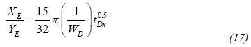
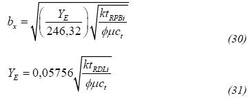
The maximum point for the case of one constantpressure boundary is governed by the following expression:
And for the case of both constant-pressure boundaries:
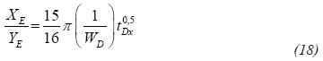
Expressions for determination of the reservoir length and area, assuming A=XEYE, is found from Equations 17 and 18, respectively:
Well off-Centered
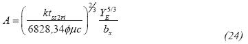
Escobar, F. H., & Montealegre, M. (2007) presented the governing equation for the unit-slope line drawn tangentially to the pressure derivative curve for constant-pressure lateral boundaries, (Figure 4):
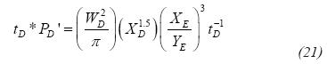
The equation for drainage area is derived from manipulation of Equations 11 and 21, assuming A=XEYE and replacing the dimensionless expressions, Equations 2-4, in the resulting equation, then:
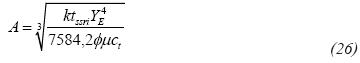
For the mixed boundary case (Figure 4) the governing equation was also presented by Escobar, Hernández & Hernández (2007) as:
By the same token:
When dual-linear and linear flow regimes are exhibited, (Figure 5), then the governing equation is:
Which leads to the following equation for estimation of the reservoir drainage area:
The maximum point in Figure 5 is governed by the following expression presented by Escobar et al. (2007).
From which the following expression area obtained:
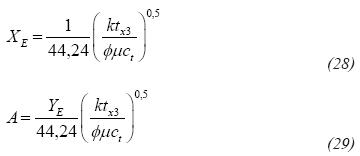
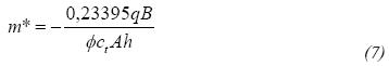
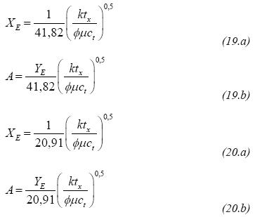
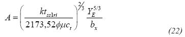
bx and YE in Equations 22 and 24 can be obtained from the equation presented by Escobar et al. (2007) using the TDS technique:
Or from the conventional straight-line method, Escobar & Montealegre (2007):
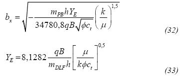
The just mentioned references contain some other expression to estimate well position and reservoir width along with the estimation of the geometric skin factors.
A practical summary of the drainage area equations is provided in Table 1.
EXAMPLES
Synthetic Example 1
A drawdown test was generated for a circular (re=1000 ft) constant-pressure reservoir with the information given in Table 1. Figure 6 contains the pressure and pressure derivative data for this synthetic test. Find reservoir drainage area.
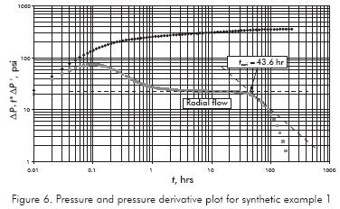
Solution. For this reservoir, the drainage area is (πx10002) = 3 141 593 ft2. From Figure 6, the intercept, tssri, of the minus-one slope straight with the radial flow regime line takes place at 43,6 hr. Using this value in Equation 12 the obtained area is 3 074 103 ft2 which is a reasonable value for this case. Other estimations are reported in Table 3, including that from Equation 7. For this case, the cartesian slope was found using the latest points in the test.
Synthetic Example 2
Figure 7 shows the pressure and pressure derivative plot for a well centered inside a rectangular reservoir with a no-flow lateral boundary and a constant-pressure boundary. Data used for the simulation are given in the Table 2. Find reservoir drainage area.
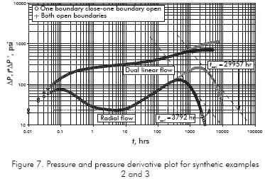
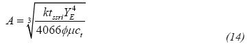
Solution. From Figure 7, tssri = 29,957 hr. The resulting area value from Equation 14 along with others is reported in Table 2.
Synthetic Example 3
Figure 7 also shows the pressure and pressure derivative plot for a well centered inside a rectangular reservoir with constant-pressure lateral boundaries. This simulation was attained using data from the third column of Table 2. Find reservoir drainage area.
Solution. From Figure 7, tssri = 3,792 hr and the maximum point, tx = 501 hr. The results from Equations 16 and 20b are reported in Table 3, along with some others.
Synthetic Example 4
A drawdown test was generated for a well centered inside a rectangular-shaped reservoir with one constantpressure boundary and one no-flow boundary, using the information given in Table 1. Figure 8 contains the pressure and pressure derivative data for this synthetic test. Find reservoir drainage area.
Solution. From Figure 8, tss2ri = 5,600 hr and tx = 2001 hr. The results from Equations 24, 19b, 7 and 8 are also reported in Table 3.
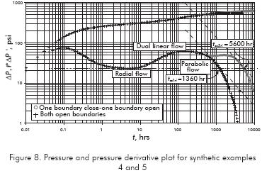
Synthetic Example 5
Contrary to Example 4, in this example the reservoir has both contant-pressure lateral boundaries. Needless to say that the simulation was performed with data from Table 1. The pressure and pressure derivative plot is given in Figure 8. Find reservoir drainage area.
Solution. From Figure 8, tss1ri = 1,360 hr. The result from Equation 22 along with others is reported in Table 3.
Synthetic Example 6
A simulation with the information from Table 1 was run for a well inside a long reservoir, near a no-flow boundary and far from the contant-pressure boundary is presented in Figure 9. Find reservoir drainage area.
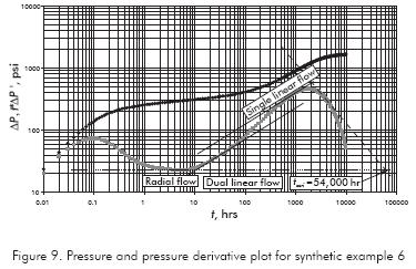
Solution. Since the well is off-centered in a rectangular reservoir and the open boundary is far from the well, then, both dual-linear and single-linear flow regimes are observed. From Figure 9, tssri = 54 000 hr, then the reasonreservoir drainage area estimated from Equation 26 is 3 878 150 ft2. Other results are provided in Table 3.
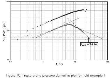
Field Example 1
Escobar et al. (2007) reported a drawdown test run in a channelized reservoir in the Colombian Eastern Planes basin. Reservoir and well parameters are given in Table 2. Dimension parameters in Table 2 were obtained from the reference. The initial pressure is 1326,28 psi and the pressure and pressure derivative data are reported in Figure 11. Estimate reservoir drainage area.
Solution. From Figure 10, tssri = 24 hr. A reservoir drainage area of 474 880,2 ft2 was obtained from Equation 22. A reservoir width of 355 ft was also obtained from a commercial software since it was not practical to obtained an acceptable match for this test.
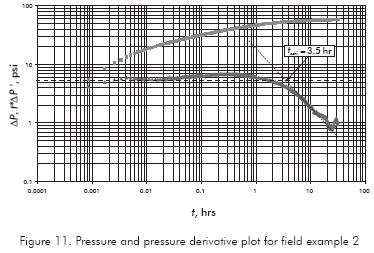
Field Example 2
Figure 11 presents the pressure and pressure derivative plot for a test run in a well in the Colombian Eastern Planes basin. The well-flowing pressure for this test is 1527,36 psi. Other information pertienent to this pressure tests is given in Table 2. Find reservoir drainage area.
Solution. From Figure 11, tssri = 3,5 hr is used in Equation 12 to provide an area of 335 164 ft2 and 314 984 ft2 from Equation 8. The reservoir geometry looks to be slightly rectangular (although a faulted reservoir may be considered). For this test was difficult to obtain a reasonable match using a rectangular geometry. The best match was obtained for a circular reservoir with a radius of 278 ft which gives an area of 242 696 ft2.
Field Example 3
Pressure and pressure derivative from a DST data run in a well located in the High Magdalena River Valley basin in Colombia are reported in Figure 12. The well-flowing pressure for this well is 429,08 psi. Other important data related to this test is given in Table 2. Find reservoir drainage area.
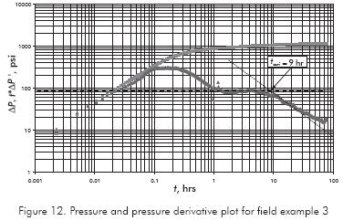
Solution. A value of tssri of 9 hr is read from Figure 12 and used in Equation 12 to estimate an area of 147 030 ft2. The best match obtained for this test was for a circular reservoir model with a radius of 210 ft. This gives an area of 136 544 ft2 using a commercial simulation which closely agrees with the equation proposed here.
ANALYSIS OF RESULTS
From the worked examples, especially the simulated ones, is oberved that the late-time pseudosteady-state equation for conventional cartesian analysis performs poorly for rectangular- shaped reservoirs having one or both lateral boundaries subject to constant pressure. The TDS technique solution for pseudosteady-state provide approximated area estimations in circular/ square constant-pressure reservoirs.
In the worst case, the introduced equations provided an absolute error of 11,3% in the estimation of the reservoir area. However, care should be taken in the selection of the appropriate equation which are easily summarized in Table 1. Of course, the proposed equations which are based upon the TDS technique are dependant on the quality of the pressure derivative curve.
CONCLUSIONS
- New equations for estimating reservoir drainage area in steady-state systems have been presented and successfully tested with synthetic and field examples. It was found that the pseudosteady-state cartesian solution fails to provide accurate results of the reservoir drainage area, especially in rectangular-shaped reservoirs. The pseudosteady-state solution of the TDS technique performs better and may be applied in either square- or circular-shaped reservoirs.
REFERENCES
Chacón, A., Djebrouni, A., & Tiab, D. (2004). Determining the Average Reservoir Pressure from Vertical and Horizontal Well Test Analysis Using the Tiab's Direct Synthesis Technique. Paper SPE 88619 presented at the SPE Asia Pacific Oil and Gas Conference and Exhibition held in Perth, Australia, 18-20, October 2004. [ Links ]
Escobar, F. H., Hernández, Y. A., & Hernández, C. M. (2007). Pressure Transient Analysis for Long Homogeneous Reservoirs using TDS Technique. J. Petrol. Sci. Eng., 58, Issue 1 (2): 68-82. [ Links ]
Escobar, F. H., & Montealegre, M. (2007). A Complementary Conventional Analysis For Channelized Reservoirs. CT&F - Ciencia, Tecnología y Futuro. 3 (3): 137-146. [ Links ]
Ramey, H. R., Jr., & Cobb, W. M. (1971). A general Buildup Theory for a Well in a Closed Drainage Area. JPT Dec. 1971: 1493-1505. [ Links ]
Tiab, D. (1993). Analysis of Pressure and Pressure Derivative without Type-Curve Matching: 1- Skin Factor and Wellbore Storage. Paper SPE 25423 presented at the Production Operations Symposium held in Oklahoma City, OK, Mar. 21-23, 1993. P. 203-216. Also, J. Petrol. Sci. Eng., 12 (1995): 171-181. [ Links ]
Tiab, D. (1994). Analysis of Pressure Derivative without Type-Curve Matching: Vertically Fractured Wells in Closed Systems. J. Petrol. Sci. Eng., 11 (1994): 323-333. [ Links ]