Services on Demand
Journal
Article
 English (pdf)
 Article in xml format
 Article references
 Send this article by e-mail
Indicators
-
 Cited by SciELO
 -
 Access statistics
Related links
-
 Cited by Google
 -
 Similars in
SciELO
Similars in
SciELO -
 Similars in Google
Share

 Permalink
CT&F - Ciencia, Tecnología y Futuro
Print version ISSN 0122-5383On-line version ISSN 2382-4581
C.T.F Cienc. Tecnol. Futuro vol.4 no.4 Bucaramanga July/Dec. 2011
CFD TECHNIQUE TO CALCULATE TUBE SKIN PEAK TEMPERATURES IN REFINERY FURNACES
Fabián-Andrey Díaz-Mateus1* and Jesús-Alberto Castro-Gualdrón2*
1Ambiocoop S.A.- Piedecuesta, Santander, Colombia
2Ecopetrol S.A. - Instituto Colombiano del Petróleo (ICP), A.A. 4185 Bucaramanga, Santander, Colombia
E-mail: fabian.diaz@ecopetrol.com.co jesus.castro@ecopetrol.com.co
(Received Jul. 25, 2011; Accepted Nov. 11, 2011)
*To whom correspondence should be addressed
ABSTRACT
Tube skin peak temperature is one of the major parameters in furnaces operation since they determine the life of the tubes and the extent of an operation run. This parameter is very difficult to calculate appropriately in magnitude and location within the furnace, and commercial furnace simulators usua-lly fail in its calculation. Computational fluid dynamics (CFD) is the only technique that calculates peak skin temperatures with great precision and accuracy since radiation and convective heat fluxes can be calculated taking into account every singularity of the geometry of the furnace and the burners. In this work, a technique is developed to calculate this parameter using CFD commercial code (Ansys Fluent) and an in-house furnace simulator (EcoFursim©). When results of the simulations are compared to data from different furnaces from Barrancabermeja refinery (Barrancabermeja, Colombia), a good agreement is observed. Refinery furnace is referred in this paper to fired heaters for non reacting heat up of hydrocarbons or petroleum crude.
Keywords: Multi-zone method, Furnace simulator, Heat fluxes, Radiation, Flame, Refinery Furnaces, Simulation, Software, Fluid Flow, Burners, Fluid Flow, Burners.
RESUMEN
Las temperaturas pico de piel de tubo es uno de los principales parámetros que se controlan en la operación de hornos industriales ya que determinan la vida de los tubos y la extensión de una corrida de operación. Este parámetro es muy difícil de calcular con precisión y los simuladores comerciales de hornos suelen fallar en su cálculo. Dinámica computacional de fluidos (CFD) es la única técnica que calcula temperaturas pico de piel de tubo con gran precisión y exactitud ya que los flujos de calor irradiativos y convectivos pueden ser calculados tomando en cuenta cada particularidad en la geometría de los hornos y los quemadores. En este trabajo se desarrolla una técnica para calcular este parámetro usando código CFD comercial (AnsysFluent) y un software simulador de hornos propio (EcoFursim©). Los resultados son comparados con datos de hornos de la refinería de Barrancabermeja (Barrancabermeja, Colombia) y se observa buena concordancia. En esta publicación, los hornos de refinería se refieren a calentadores por fuego directo para el calentamiento no reactivo de hidrocarburos o petróleo.
Palabras claves: Método multizona, Simulador de hornos, Flujos de calor, Radiación, Llama, Hornos de refinería, Simulación, Software, Dinámica de fluidos, Quemadores.
RESUMO
As temperaturas pico de pele de tubo é um dos principais parâmetros que são controlados na operação de fornos industriais já que determinam a vida dos tubos e a extensão de uma corrida de operação. Este parâmetro é muito difícil de calcular com precisão e os simuladores comerciais de fornos acostumam falhar em seu cálculo. Dinâmica computacional de fluidos (CFD) é a única técnica que calcula temperaturas pico de pele de tubo com grande precisão e exatidão já que os fluxos de calor irradiativos e convectivos podem ser calculados considerando cada particularidade na geometria dos fornos e dos queimadores. Neste trabalho é desenvolvida uma técnica para calcular este parâmetro usando código CFD comercial (AnsysFluent) e um software simulador de fornos próprio (EcoFursim©). Os resultados são comparados com dados de fornos da refinaria de Barrancabermeja (Barrancabermeja, Colômbia) e uma boa concordância é observada. Nesta publicação, os fornos de refinaria se referem a aquecedores por chama direta para o aquecimento não reativo de hidrocarbonetos ou de petróleo.
Palavras-chaves: Método multi-zona, Simulador de fornos, Fluxos de calor, Radiação, Chama, Fornos de refinaria, Simulação, Software, Dinâmica de fluidos, Queimadores.
1. INTRODUCTION
Tube skin temperature is one of the key parameters to be controlled in industrial furnaces operation since they determine the life of the tubes and the extent of an operation run. Furnaces tubes may rupture when skin temperatures are above the limit given by the metallurgy of the material, which is usually 1 200°F (922,05K) for 5 Cr - 0,5 Mo steels. A rupture of tubes in operation is one of the worst scenarios that a process engineer could face; hence, proper calculation of tube skin peak temperature is probably the most important parameter that a simulation of a furnace should accomplish.
The most traditional method to simulate industrial furnaces has been the multi-zone method (Hottel, 1974) and it is used by most of the commercial furnace simulators. The reason for its popularity is the efficacy to calculate mean heat fluxes and its simplicity, which makes it ideal for implementation in a complete programming code for furnaces simulation. The multi-zone has been very popular in the last 30 years, but with the rise of the CFD codes and multi-core computers, it has become obsolete.
In the multi-zone method, furnaces are divided into zones of equal properties, small singularities of the geo-metry are difficult to be taken into account with the zones and many approximations must be made. Tubes must be replaced for an equivalent plane surface and its emissi-vity is calculated by equations based on geometric factors. The fluid-dynamics and combustion patterns of the flame must be previously known; therefore, empirical equations or experimental data must be available. Given the simplifications involved in the multi-zone, mean heat fluxes are properly calculated, but peak heat fluxes usually not.
In order to calculate tube skin temperatures, most commercial furnace simulators use the API 530 “Calculation of Heater-Tube Thickness in Petroleum Refineries” or similar techniques. In the API 530, peak heat fluxes are estimated from circumferential factors taken from curves based on the work of Hottel (McAdams, 1954). These curves are not available for shield tubes where very often peak skin temperatures are found.
All these difficulties previously mentioned are overcome with CFD simulation. The geometries can be built exactly and fluid-dynamics and combustion patterns of the flame can be calculated with different methods available in commercial CFD codes; also, convective and radiative heat fluxes can be calculated in detail. CAD (Computer Aided Design) geometries of furnaces can be meshed into millions of cells depending upon the computational resources available, but with a multi-core computer or cluster, plenty of RAM memory and parallel computing, large industrial furnaces can be simulated even when the gas tips are several times smaller than the furnace itself, demanding a lot of mesh to be properly modeled.
EcoFursim© is an in-house furnace simulator deve-loped at the Ecopetrol S.A. - Instituto Colombiano de Petróleo (ICP). It uses the multi-zone method and the API 530 to calculate heat fluxes and tube temperatures, respectively. EcoFursim© is specialized in hydrocarbon and petroleum simulation, it has its own characterization package and thermodynamic package. For more detailed information, see Díaz and Castro (2010). EcoFursim© is necessary as a starting point for the CFD simulations developed in this work because the furnaces simulated charge hydrocarbon or petroleum feeds and CFD commercial codes are not the best tool available for hydrocarbon simulation, as it will be explained further in this paper.
After many simulations of refinery furnaces deve-loped with EcoFursim©, it was found that mean heat fluxes are responsible to heat up the feed. Since they are properly calculated with the multi-zone method, outlet temperatures of the feed are also properly calculated. (Díaz & Castro, 2010). However, based on real data, it was found that tube skin peak temperatures were not a-ccurately calculated with the multi-zone method, neither in location nor in magnitude within the furnace. Therefore, CFD is the only technique available to accurately calculate this parameter, considered by the authors as the main goal that a simulation of an industrial furnace should accomplish. The authors did not find publications on CFD simulation of refinery furnaces focused on tube temperatures, since most of the research available in the literature on CFD simulation of furnaces has been performed on cracking furnaces such as Heynderickx, Oprins, Marin, and Dick (2001), Oprins and Heynderickx (2003), Stefanidis, Merci, Heynderickx and Marin (2006), Habibi, Merci and Heynderickx (2007), Stefanidis, Merci, Heynderickx and Marin (2007),
Arrieta, Cadavid and Amell (2011). In these studies, the combustion in the furnaces was simulated in CFD using different combustion and radiation models, but the tube skin temperatures were calculated by a different source rather than the CFD model itself. This separate source is commonly a computer code where all the cracking reactions are modeled, and physical properties and tube skin temperatures are calculated. This temperature is the same for the entire perimeter of the tube; it means there are not peak or medium skin temperatures. This is a good approach for cracking furnaces where tubes receive practically the same radiation from all sides. However, most refinery furnaces, as those simulated in this work, have refractory backed tubes and the incident radiation can be several times bigger in the point where the tube faces the flame. A clear graph of incident radiation on tubes can be found in Hewitt, Shires and Bott (1994). The main objective of this work is to propose a technique to calculate tube skin peak temperatures in refinery furnaces. In order to accomplish this objective, the CFD model calculates the skin temperature through the entire perimeter of the tube, and the temperature and the heat transfer coefficients of the fluid are calculated by a different source (EcoFursim©).
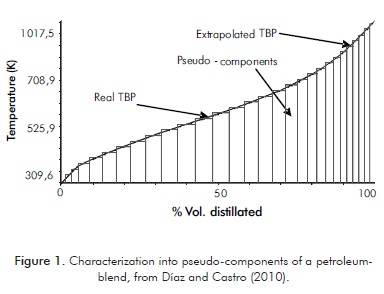
The petroleum crude is simulated by a mixture of characterized pseudo-components or cuts. These are calculated from the partition of the TBP curve (True Boiling Point) as on Figure 1. Densities are calculated through the KW and the rest of the properties of the cuts are calculated with correlations such as API TDB (1997), Aladwani and Riazi (2005) and Twu (1984). A thermodynamic package is necessary to calculate the VLE (Vapor Liquid Equilibrium) and the properties of this multi-component mixture. This complex procedure is finely executed by commercial process simulators as well as EcoFursim©. To implement this procedure in a CFD code can be extremely complicated and unnece-ssary if the previously mentioned tools are available. Besides, not simulating petroleum in CFD is an important reduction in computational effort.
Experimental tube skin temperatures presented in this work were measured with a FLIR P50 F NTSC thermographic camera with an emissivity of 0,85 and a distance of 10 m, measurement errors are ± 2°F. Experimental gas temperatures were measured with thermocouples installed within the furnaces. Recommended practices used for temperature measurements in furnaces were taken from the API 573 “Inspection of fired boilers and heaters”.
2. CFD TECHNIQUE TO SIMULATE FURNACES
Meshing
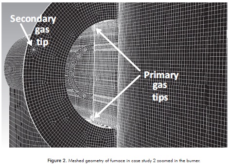
Computational resources available are a key issue when simulating in CFD. Due to the huge size that industrial furnaces have and the miniature size of the gas tips, meshes for this kind of simulations often have over 1 million cells. In order to reduce the size of the meshes, the authors the symmetric characteristics of furnaces must be taken advantage of. It is a good practice to isolate the burners from the radiation chamber and connect them by a non-conformal mesh interface. In this way, the radiation chamber can be meshed with structured hexahedrons and the burners with unstructured cells of any form. However, in the interface it is recommended to maintain the variation in size of the elements between 1 - 1,2 to avoid interpolation errors. In Figure 2, the meshed geometry and the interface between the burner and the radiation chamber of one of the furnaces simulated in this work is observed. For better clarity of the full geometry of this furnace, see Figure 9.
Boundary conditions
When the CAD geometry of the furnace is built a hole is left in the place where the tubes are located, the remaining wall boundary would be the surface of the tubes. Boundary conditions at this wall must be carefully selected and calculated since tube skin temperature is a highly sensible parameter and diffi cult to calculate accurately. Many factors intervene in its calculation such as fouling, heat transfer coeffi cient, coke deposition, etc. The boundary conditions to be provided to the simulation are as follows:
- Heat transfer coefficient.
- Temperature.
- Emissivity (0,94 for clean new tubes, 0,85 for fouled old tubes).
- Wall thickness.
The bulk temperature of the fl uid can be provided to the simulation as boundary condition but not the fluid film heat transfer coefficient. It must be treated to include the effect of fouling, wall thickness and coke deposition; Equations 1 to 4 can be used.
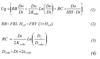
Equation 2 is for two-phase flows and it should be used in case of wave, stratified or slug flow patterns. For Bubble, plug, froth or annular patterns, use only the fouling resistance of the liquid. For mist, use only the fouling resistance of the vapor.
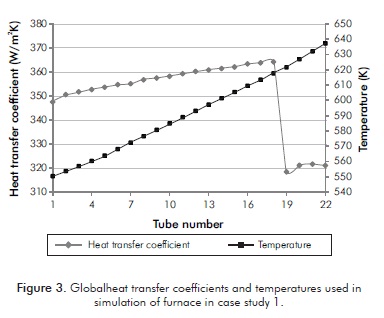
In this work inside fi lm heat transfer coefficients and fluid temperatures were calculated with the soft- ware EcoFursim© and used in the equations proposed. Fouling resistance is a parameter difficult to determine and is purely empiric. Based on experimental data and CFD simulations, for light hydrocarbons and gases, we recommend the value of 0,0005 m2.K/W - 0,0006 m2.K/W. For heavy hydrocarbons, we recommend 0,001 m2.K/W - 0,002 m2.K/W in tubes with operation time over 2 0 000 hours. These fouling resistances are based on data from Thome (2010). For the refractory walls, the outside heat transfer coefficient can be calculated with Churchill's (1983) method for natural convection. Figure 3 presents global heat transfer coefficients obtained by Equations 1 to 4 using inside film heat transfer coefficients and temperatures calculated with EcoFursim©.
Fluid flow
The equations that describe the three dimensional stationary fluid flow in furnaces are RANS based (Reynolds Average Navier Stokes), the flow can be considered incompressible since high Mach numbers are not presented. The realizable k-ε model (Shih, Liou, Shabbir & Zhu, 1995) can be used for proper turbulence modeling since there are not severe pressure gradients or strong streamline curvatures although moderate swirl is expected.
The realizable k-ε differs from the standard k-ε in the calculation of μt and the transport equation of ε, this yields superior performances in swirling flows. Equations 5 to 9 describe conservation of mass and momentum, energy and turbulence modeling.
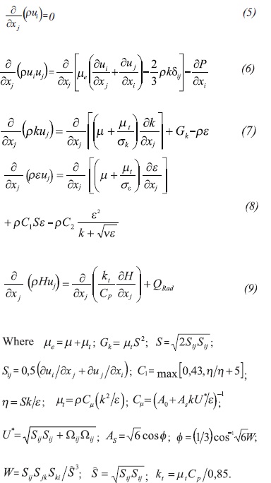
The constants for the realizable k-ε are:A0 = 4,04; C1ε =1,44; C2=1,9; σK=1,0; σε=1,2. The realiza-ble, as well as the other k-ε models, requires maintai-ning the y+ coefficient between 30 - 300 in order to use the standard wall functions as proposed by Launder and Spalding (1974). Thus, the cells at the walls were rigorously sized to fulfill this constraint.
Combustion
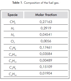
The mathematical model selected for non premixed turbulent combustion modeling was the PDF/mixture fraction (Probability Density Function). The mixture fraction is a good approach for turbulent flows where turbulent convection overwhelms molecular diffusion. Other models such as Finite Rate and Eddy Dissipation can be used for non-premixed combustion but they require solving one equation for each specie involved in the combustion; being the fuel gas a mixture of different gases (See Table 1), the number of equations would generate a giant computational effort. On the other hand, with the mixture fraction only two equations have to be solved, one for the mean mixture fraction and one for the mixture fraction varianceand all of the species mass fractions, density and temperature are contained in a PDF table (Cant & Mastorakos, 2008). As the compositions of the species are calculated at equilibrium, incomplete combustion and intermediate species are not properly calculated, but temperatures and flame patterns are, as it is needed in this work. Equations 10 and 11 describe the mixture fraction model.
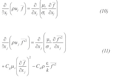
Where  and the constants σi = 0,85; Cg =2,86; Cd = 2,0. Balances for every single component involved in the combustion are not necessary since the instantaneous values of mass fractions, density, and temperature depend solely on the instantaneous mixture fraction (Ansys Fluent, 2011), see Equation 12.

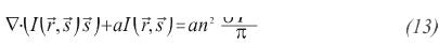
Radiation In order to calculate accurate skin temperatures, heat fluxes have to be accurately calculated; therefore, (Discrete ordinates) DO was selected since it is the more rigorous radiation model available; besides, DO suits for all the range of optical thickness. Equation 13 is the no scattering, gray gas DO radiation model.
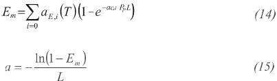
The products of combustion CO2 and H2O are not transparent to radiation and must be included in the emissivity of the mixture of gases, Equation 14. This is calculated with the weighted-sum-of-gray-gases model (WSGGM) as presented by Hottel and Sarofi m (1967); this is a widely accepted approach because is not as simple as the gray gas assumption, but not as complex as taking into account every gas absorption band. The absorption coeffi cient is calculated with Equation 15.
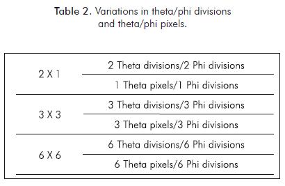
The DO model is very sensitive to the theta/phi divisions and the theta/phi pixels. The more divisions and pixels the model has, the more computationally expensive it becomes. In order to determine the opti- mal number of theta/phi divisions and theta/phi pixels, furnace in case study 2 was simulated using variations in Table 2, and tube skin temperatures calculated where compared in Figure 4.
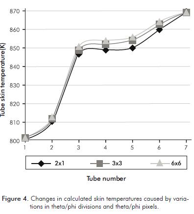
Based on Figure 4, we recommend that at least 3x3 divisions/pixels in the DO radiation model should be used in simulations where tube skin temperatures need to be accurately calculated.
Numerical solution
The radiation chambers in the furnaces simulated were meshed with hexahedrons. As a result, we cons- tructed a grid which is basically aligned with the flow. This allowed us to use first order upwind as discreti- zation scheme without incurring in signifi cant false diffusion (See Versteeg and Malalasekera, 1995). The discretization scheme selected to calculate the pressure term was the PREssure STaggering Option (PRESTO!) which is recommended when swirling fl ows or buo- yant effects are expected (Ansys Fluent, 2011). As the solver selected is pressure-based, the SIMPLE algorithm (Patankar, 1980) was selected as scheme for pressure- velocity coupling.
Convergence of the model
A high quality CFD simulation must be mesh- independent; in this case, the meshes were refined until calculated tube skin temperatures in the furnaces remained unaltered. Furnace in case study 1 required 1,8 million cells and furnace in case study 2 required 2,5 million cells to be mesh-independent.
The key parameter to determine the convergence of the CFD models presented in this work was the energy unbalance which was assured to be lower than 1% of the inlet energy in one burner. This goal required a lot of iterations, around 5 000 - 6000. Other parameters to check convergence such as mass unbalance, equation residuals and invariability of the calculated results will be attained if the energy unbalance is assured as already explained.
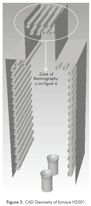
3. CASE STUDY 1: FURNACE H2001
Furnace H2001 is typical box type configuration with 12 burners located in the floor and refractory-backed radiant tubes in a single row. The 2 burners located in both end walls are not symmetrical but the remaining 10 are indeed symmetrical between each other. There- fore, only half a burner needs to be simulated, the side boundaries would be symmetry axes. These symmetry axes are already defined on Figure 5.
Furnace H2001 has two passes for the feed, but only one is simulated in EcoFursim© because both passes are expected to be equal. Tubes are numbered from top to bottom. Furnace dimensions and operating conditions are summarized in Table 3, values taken for ε coke are based on historical plant data and photograph files. Figure 6 is one of the images obtained in the thermographic study of furnace H2001 and shows the shield tube bank.
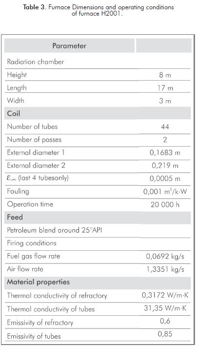
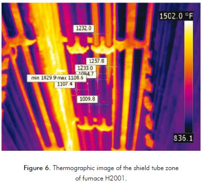
Figure 7 are the contours of temperature calculated for H2001 on the symmetry plane, tubes and furnace walls. Figure 7 is zoomed in the shield tube bank where tube skin peak temperatures are found. Results of the CFD simulation are compared with a simulation of the same furnace performed with the software EcoFursim© and real data in Figure 8 and Table 4.
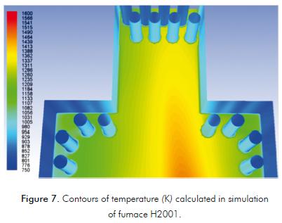
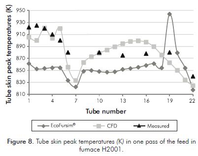
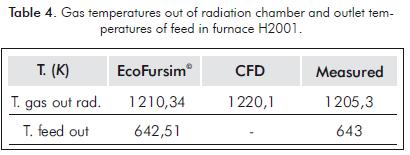
Figure 8 shows that tube skin peak temperatures cal- culated with the CFD simulation are very similar to mea- sured values with less than 2% error. However, tube skin peak temperatures calculated with EcoFursim© present a mean error of 9%; although, gas and feed temperatures are very accurate as seen on Table 4. The reason for this disparity is the peak and medium heat fl uxes calculated with the multizone method and the API 530.
In Table 5, we can see that medium heat fluxes are very similar to both computational methods. They are probably more accurate with EcoFursim©, since tem- peratures in Table 4 are closer to measured values. We can conclude two different issues: Medium heat fluxes are very well calculated with the multi-zone method, and they are in charge of heating up the crude feed, which properties are also correctly calculated with EcoFursim© thermodynamic package. Nevertheless, there is a marked difference between calculated peak heat fluxes; these were calculated with the multi-zone method and the API 530 in EcoFursim©.
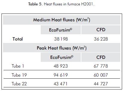
Peak heat fluxes are responsible for peak skin tem- peratures and EcoFursim© cannot properly calculate the strong radiative and convective peak heat fluxes that reach the shield tubes of furnace H2001 (tubes 1 to 6), because of two reasons: Strong convective heat fluxes are much more accurately calculated with CFD than with empirical methods available in the literature. Hottel curves in the API 530 are not available for shield tubes, and circumferential factors have to be extrapolated from similar curves.
In tube 19, a markedly strong peak heat flux is calcu- lated by EcoFursim©, related to the circumferential fac- tor estimated from Hottel curves in the API 530. Tubes 1 to 18 are 6" diameter and tubes 19 to 22 are 8" diameter. This difference in diameter causes an over-estimation of the circumferential factor, which is a function of the ratio tube spacing/tube diameter.
4. CASE STUDY 2: FURNACE H1304
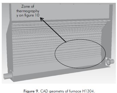
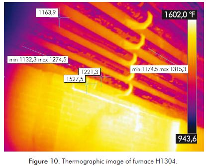
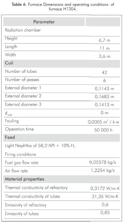
Furnace H1304 is a typical box type with 4 burners located at opposite end walls. Tubes are refractory-backed in a single row and there is no convection section. It has 6 passes for the feed; because of symmetry, only half a furnace and 3 passes are simulated. CAD geometry of furnace H1304 is in Figure 9. Furnace Dimensions and operating conditions are summarized in Table 6. Figure 10 is one of the images obtained in the thermographic study of furnace H1304, and shows the first tubes from the floor to the top. Tubes are numbered from top to bottom, thus tube 21 is the closer to the flame.
The location of tube skin peak temperatures within the furnace is clearly seen in Figure 11. One would expect the peak temperatures in the middle of the furnace, but because of fluid dynamics related to this furnace and internal characteristics, peak temperatures are found closer to the right end wall. This particular phenomenon can only be simulated with CFD.
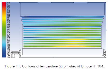
Figure 12 shows how tube skin peak temperatures are accurately calculated with CFD simulation, errors in cal- culation are below 2%. Data calculated with EcoFursim© present a mean error of 10%. All data calculated in both methods for pass 1 are very similar. This is because pass 1 is the furthest from flames and strong peak heat fluxes are not presented. However, in the last tubes a marked difference between EcoFursim© and CFD results is seen. The reason is the strong peak heat fluxes presented near the flame, which are only properly calculated in the CFD simulation.
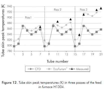
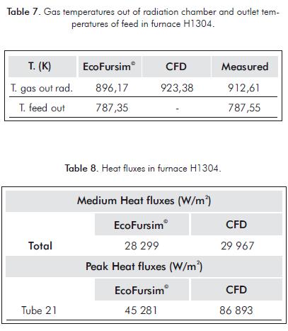
Values on Tables 7 and 8 permit to conclude the next issues: Gas temperatures and medium heat fluxes are accurately calculated with the multi-zone method in EcoFursim©. These fluxes are in charge of heating up the feed, which properties are correctly calculated with EcoFursim©. The result is an accurate calculation of feed outlet temperature. Peak heat fluxes calculated near the flame are not properly calculated with the multi-zone method and the API 530 in EcoFursim© as observed on tube 21 on Table 8. Figure 12 shows that the closer tubes are from flame, the more inaccurate peak skin temperatures are calculated.
5. DISCUSSION
The multi-zone method and the API 530 cannot properly calculate strong peak heat fluxes because of several reasons. There are many simplifications involved in the use of these methods; let's discuss the three main reasons:
- Circumferential factors: Peak heat fluxes are estimated from circumferential factors taken from Hottel curves which are available for only 4 types of tube arrangements. Significant errors are found when there are changes in tube diameter in the coil (See Figure 8).
- Flame patterns are necessary to estimate the release of heat from combustion in every zone, these patterns are difficult to obtain and are simplified to semi-empirical equations.
- Convective heat transfer correlations: These are necessary to calculate convective fluxes and are only available in the literature for a very reduced number of coil arrangements and furnace tube geometries.
- In many cases, there are small singularities of the furnace and the burners that generate localized peak heat fluxes. Singularities like this are seen on Figure 11, where peak temperatures are located closer to the right end wall of furnace H1304, and only the CFD simulation could reproduce this phenomenon.
6. CONCLUSIONS
-
Contours of temperature found in CFD simulation, as those on Figure 11, can be extremely detailed and accurate to determine the exact location of warmer spots and tube skin peak temperatures. This valuable information could be used to determine the location of thermocouples within a furnace.
-
The method proposed to calculate global heat transfer coefficients in equations 1 to 4 is very useful because the feed of the furnace does not have to be simulated in the CFD model, which is an important reduction in computational effort. Besides, all the properties necessary to calculate the heat transfer coefficients can be more accurately calculated with commercial process simulators or specialized software like EcoFursim©. The good accuracy and precision found in all the tube skin temperatures calculated in this work, demonstrates the efficacy of the technique proposed to simulate furnaces using CFD.
-
Two situations are presented in Figure 8: First, tube skin peak temperatures in shield zone (tubes 1 to 6) are correctly calculated with CFD with a mean error of 1% and inadequately calculated with EcoFursim© with a mean error of 9%. For the rest of the tubes, both simulations present a similar mean error of 3%, except for tube 19, whose overestimation in EcoFursim© was already explained. Shield tubes of furnace H2001 receive a strong heat flux, due to the length of the flames. These fluxes are calculated very different in both simulations (see table 5). EcoFursim© cannot accurately simulate the long flames and the strong convective fluxes that reach the shield tubes while the CFD simulation could, as seen on the tube skin peak temperatures.
-
The same two situations are presented in Figure 12. Tubes 1 to 10 are far from the flame and peak temperatures are similar and properly calculated in both simulations with a mean error below 1%. A diffe-rent condition is presented in tubes 17 to 21, which are closer to the flame. Peak temperatures are only properly calculated with the CFD simulation with a mean error below 2%, while EcoFursim© presented a mean error of 10%. The cause is the strong loca-lized peak heat fluxes that reach these tubes (see Table 8). EcoFursim© cannot accurately simulate the deviation of the flames found in H1304 that caused a localized peak heat flux while the CFD simulation could reproduce this phenomenon which can be seen on Figure 11.
-
The Hottel multi-zone method is extremely useful to calculate medium heat fluxes and gas temperatures. Because medium heat fluxes are in charge of heating up the feed, outlet temperatures are usually accurately calculated. The API 530 method is very useful to calculate peak skin temperatures when strong peak heat fluxes are not presented. In the case of tubes with strong heat fluxes, the multi-zone method and the API 530 are not recommended by the authors of this work; errors in calculations around 10% should be expected. The CFD technique exposed in this work is recommended if the purpose of the simulation is to calculate accurate tube skin peak temperatures.
-
EcoFursim©, as well as other commercial furnace simulators, does not have the proper mathematical models to calculate accurate tube skin peak temperatures found in furnaces when tubes are reached by strong peak heat fluxes. Deviation of the flames, internal temperature unbalance, localized flow of gases, or similar singularities that are beyond the capabilities of the multizone method,can be calculated with CFD simulation.
ACKNOWLEDGMENTS
The authors want to thank engineers Martha Yolanda Morales, Lilia Yaneth Quiroga, Manuel Julian Ardila and Luis Eduardo Navas from Barrancabermeja Refinery (Barrancabermeja, Colombia) for their support in the acquisition of mechanical and process data necessary to simulate the furnaces presented in this publication. Finally, the authors gratefully acknowledge Ecopetrol S.A. - Instituto Colombiano del Petróleo (ICP), for the financial support that allowed the development of this work.
REFERENCES
Aladwani, H. A. & Riazi, M. R. (2005). Some guidelines for choosing a characterization method for petroleum fractions in process simulators. Chem. Eng. Res. Des., 83 (2), 160 -162. [ Links ]
Ansys Fluent 13 User's Guide (2011). Canonsburg, Pennsylvania, USA. ANSYS, Inc. [ Links ]
API Technical Data Book - Petroleum Refining. (1997). American Petroleum Institute, 6Th. edition. [ Links ]
Arrieta, A., Cadavid, F. & Amell, A. (2011). Simulación numérica de hornos de combustión equipados con quemadores radiantes. Ing. Univ. Bogotá, 15 (1), 9 - 28. [ Links ]
Cant, R. S. & Mastorakos, E. (2008). An introduction to turbulent reacting flows. London: Imperial College Press. [ Links ]
Churchill, S.W. (1983). Free convection around immersed bodies. Heat Exchanger Design Handbook (2.5.7), New York: Hemisphere. [ Links ]
Diaz, F. A. & Castro, J. A. (2010). Mathematical model for refinery furnaces simulation. CT&F - Ciencia, Tecnología y Futuro, 4 (1), 89 - 99. [ Links ]
Habibi, A., Merci, B. & Heynderickx, G. J. (2007). Impact of radiation models in CFD simulations of steam cracking furnaces. Comp. Chem. Eng., 31 (11), 1389 - 1406. [ Links ]
Hewitt, G. F., Shires, G. L. & Bott, T. R. (1994). Process Heat transfer. CRC Press. [ Links ]
Heynderickx, G. J., Oprins, A. J. M., Marin, G. B. & Dick, E. (2001). Three-Dimensional Flow Patterns in Cracking Furnaces with Long-Flame Burners. AIChE Journal, 47 (2), 388 - 400. [ Links ]
Hottel, H. C. & Sarofim, A. F. (1967). Radiative transfer. New York: McGraw Hill. [ Links ]
Hottel, H. C. (1974). First estimates of industrial furnace performance, the one-gas-zone model re-examined. Heat Transfer in Flames, 5 - 28. [ Links ]
Launder, B. E. & Spalding, D. B. (1974). The numerical computation of turbulent flows. Computer Methods in Applied Mechanics and Engineering, 3 (2), 269-289. [ Links ]
McAdams , W. H. (1954). Heat transmission. (3rd. ed.), New York: McGraw-Hill. [ Links ]
Oprins, A. J. M. & Heynderickx, G. J. (2003). Calculation of three-dimensional flow and pressure fields in cracking furnaces. Chem. Eng. Sci., 58 (21), 4883 - 4893. [ Links ]
Patankar, S. V. (1980). Numerical Heat transfer and fluid flow. New York: Hemisphere. [ Links ]
Shih, T. H., Liou, W. W., Shabbir, A. & Zhu, J. (1995). A new k -e model eddy viscosity model for high Reynolds number turbulent flows model development and validation. Comput. Fluids., 24 (3), 227 - 238. [ Links ]
Stefanidis, G. D., Merci, B., Heynderickx, G. J. & Marin, G. B. (2006). CFD simulations of steam cracking furnaces using detailed combustion mechanisms. Comp. Chem. Eng., 30 (4), 635 - 649. [ Links ]
Stefanidis, G. D., Merci, B., Heynderickx, G. J. & Marin, G. B. (2007). Gray/nongray gas radiation modeling in steam cracker CFD calculations. AIChE Journal, 53 (7), 1658 - 1669. [ Links ]
Thome, J. R. (2010). Engineering Data Book III. Wolverine Tube Inc. [ Links ]
Twu, C. H. (1984). An internally consistent correlation for predicting the critical properties and molecular weights of petroleum and coal-tar liquids. Fluid phase equilibria, 16 (2), 137 - 150. [ Links ]
Versteeg, H. K. & Malalasekera, W. (1995). An introduction to computational fluid dynamics: The finite volume method. England: Longman scientific & technical. [ Links ]
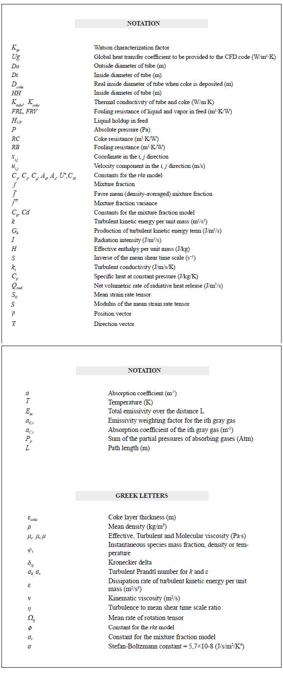
NOTATION