Services on Demand
Journal
Article
 English (pdf)
 Article in xml format
 Article references
 Send this article by e-mail
Indicators
-
 Cited by SciELO
 -
 Access statistics
Related links
-
 Cited by Google
 -
 Similars in
SciELO
Similars in
SciELO -
 Similars in Google
Share

 Permalink
CT&F - Ciencia, Tecnología y Futuro
Print version ISSN 0122-5383On-line version ISSN 2382-4581
C.T.F Cienc. Tecnol. Futuro vol.4 no.4 Bucaramanga July/Dec. 2011
NUMERICAL SIMULATION OF HIGH PRESSURE BURNER WITH PARTIALLY PREMIXED FLAME
Juan-Camilo Lezcano-Benítez1, Daniel Correa-Restrepo1, Andrés-Adolfo Amell-Arrieta1 and Francisco-Javier Cadavid-Sierra1*
1Grupo de Ciencia y Tecnología del Gas y Uso Racional de la Energía, Universidad de Antioquia, Medellín, Antioquia, Colombia
E-mail: fcadavid@udea.edu.co
(Received May. 31, 2011; Accepted Oct. 26, 2011)
*To whom correspondence should be addressed
ABSTRACT
In this paper we present the results of a 2D axisymmetric parametric study which simulates an atmospheric premixed burner with flame at high pressure, in which methane is burned. A total of nine simulations are performed with different regulators openings of primary and secondary air. Also, it provides a 3D simulation in which entry conditions are the profiles obtained in a 2D axisymmetric simulation, with the intention to note that differences are obtained between 2D and 3D simulation. The simulations are performed using the standard k-emodel for turbulence, P1 model for radiation and the Finite Rate/Eddy Dissipation model with a simplified 2-step reaction mechanism for combustion. We conclude that when the secondary air regulator is closed, combustion is incomplete. Also, the results of 2D axisymmetric are a good approximation in regards to 3D results.
Keywords: Atmospheric burner, FLUENT, Internal recirculation, Semi-spherical flame, Mathematical models, Premixed flame, Regulators, High pressure, Numerical simulation.
RESUMEN
En este trabajo se presentan los resultados obtenidos de un estudio paramétrico en 2D axisimétrico donde se simula un quemador atmosférico con llama de premezcla a alta presión, en el cual se quema metano. Son realizadas en total nueve simulaciones con diferentes aperturas de los reguladores de aire primario y secundario. También es realizada una simulación 3D que tiene como condiciones de entrada los perfiles obtenidos en una de las simulaciones 2D axisimétrica, con el fin de observar que diferencias se obtienen entre la simulación 2D y 3D. Las simulaciones son realizadas utilizando el modelo k-e estándar para la turbulencia, el modelo P1 para la radiación y para la combustión se utilizó el modelo Finite Rate/Eddy dissipation con un mecanismo reaccional simplificado de 2 pasos. Se concluye que cuando el regulador de aire secundario se encuentra cerrado la combustión es incompleta, y además los resultados obtenidos en 2D-axisimétrico son una buena aproximación con respecto a los resultados en 3D.
Palabras claves: Quemador atmosférico, FLUENT, Recirculación interna, Llama semiesférica, Modelos matemáticos, Llama premezclada, Reguladores, Alta presión, Simulación numérica.
RESUMO
Neste trabalho são apresentados os resultados obtidos de um estudo paramétrico em 2D axissimétrico onde é simulado um queimador atmosférico com chama de pré-mistura a alta pressão, no qual é queimado metano. São realizadas em total 9 simulações com diferentes aberturas dos reguladores de ar primário e secundário. Também é realizada uma simulação 3D que tem como condições de entrada os perfis obtidos em uma das simulações 2D axissimétrica, com o fim de observar que diferenças são obtidas entre a simulação 2D e 3D. As simulações são realizadas utilizando o modelo k-e padrão para a turbulência, o modelo P1 para a radiação e para a combustão foi utilizado o modelo Finite Rate/Eddy dissipation com um mecanismo reaccional simplificado de 2 passos. É possível concluir que quando o regulador de ar secundário está fechado a combustão é incompleta, e, além disso, os resultados obtidos em 2D-axissimétrico são uma boa aproximação com relação aos resultados em 3D.
Palavras-chaves: Queimador atmosférico, FLUENT, Recirculação interna, Chama semi-esférica, Modelos matemáticos. Llama pré-misturada, Reguladores, Alta pressao, Simulacao numérica.
1. INTRODUCTION
This work proposes the simulation of a furnace used in the refining industry.
The simulation aims to obtain important furnace operating parameters to allow enhanced furnace production. In order to simplify the furnace simulation, the problem is divided in two stages: the first covers the simulation of a furnace burner which results are taken into the second stage to be used as input conditions to simulate the furnace itself. The work of taking the burner results and developing the furnace simulation was made by Arrieta, Cadavid and Arrieta (2011). The currently work involves the first stage, i.e. only the burner simulation.
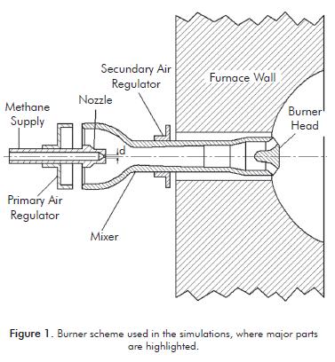
In this work, the most important burner features are shown: first of all, it is a partially premixed atmospheric burner where the combustion air is entrained from the environment by a high-speed jet. Figure 1 shows a scheme of this burner with its main parts, where a high pressure methane jet is discharged from the nozzle into the venturi or mixer, causing the effect of decreasing the pressure within itself, therefore dragging ambient air that is at atmospheric pressure. The amount of air entering the mixer is regulated by the primary air obturator with an axial displacement. Then the mixture of methane and air moves toward the burner head, being discharged into the furnace where the flame takes place. The air required to complete combustion is entrained from the external environment by the flame and regulated with the secondary obturator. As shown in Figure 1, the discharged of the fuel-air mixture in the burner head is made tangentially on a dome carved into the furnace wall, which gives stability to the flame and causes it to be shorten and with tendency towards a spherical shape.
Although current simulations involving turbulence tend to be modeled with Large Eddy Simulation (LES), models involving Reynolds Average Navier-Stokes (RANS) equations remain as the preferred tool for modeling industrial applications due to lower computational demand that is required by the latter.
Among recent works developed to simulate turbulent flames involving RANS models, the one elaborated by Herrmann (2006) simulated three methane Bunsen burners which differ only in the Reynolds number. In his paper he uses the turbulence model of two equations standard k-ε, and finds the concentration of chemical species through a probability density function (PDF). The results obtained are acceptable in comparison to experimental data. Jiang, Liang, Huang and Li (2006) conducted a simulation of a diffusion flame of CH4 /air, for which three different turbulence models are used (k-ε realizable, k-ω, and the Reynolds Stress Model) finding that the best results are obtained with the k-ω model. Bidi, Hosseini and Nobari (2008) simulated a premixed flame of CH4/air in a cylindrical combustion chamber using the k-ε standard model. The reaction rates are found with the Finite Rate/Eddy Dissipation model with a 5 step reactional mechanism, taking into account the effect of radiation by using the Discrete Ordinate Method (DOM). The absorption coefficient is also calculated by using a weighted sum of gray gases (WSGGM), obtaining results that are in excellent agreement with experimental outcomes.
The standard k-ε model is generally good, but when the flow is restricted by a wall, results lose accuracy, whereas the k-ω model is better when the wall is present (Roy & Blottner, 2006). Despite this, the standard k-ε model is widely used due to its simplicity.
In this work we use the commercial software FLUENT 6.2.16 to study the behavior of the burner shown in Figure 1, using methane as fuel. First, the study develops a parametric 2D axisymmetric model in which different primary and secondary regulators openings are simulated. Also, the simulation of a 3D model is performed, using as input conditions the results obtained from a 2D axisymmetric simulation.
2. 2D-AXISYMMETRIC MODEL
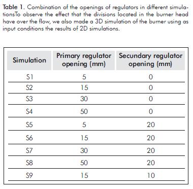
It can be considered that both the burner and the flow have rotational symmetry around its axis, but the burner head has divisions which doesn´t make it axisymmetric. However, since the divisions are small in size, its effect is considered not significant and, therefore, a 2D axisymmetric burner model is developed. To observe the burner behavior, several simulations in two dimensions were performed by modifying the opening of primary and secondary air regulators, as shown in Table 1.
Operating Conditions
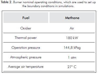
In Table 2, the burner operating conditions are shown, which are useful to determine boundary conditions at the simulations.
All 2D-axisymmetric simulations have a maximum Mach number around 1,19, which is obtained when the fuel is discharged from the nozzle into the mixer, implying that the flow in this zone is supersonic. To suppose that a gas flow is compressible, we use a criterion where the Mach number should be higher than 0,1, because below this value the density variation in function of pressure can be ignored. In these simulations, the flow must be considered compressible.
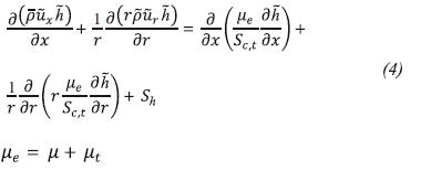
Governing Equations
Equations for a compressible, turbulent and reactive flow in 2D axisymmetric are shown below. The flow is considered compressible because the methane is discharged in the nozzle at supersonic speed, genera-ting a large pressure gradient in this area. The equations governing the problem are the complete Navier Stokes equations, i.e. augmented by the laws of chemical kine-tics, measured with the Favre average, which takes into account the density fluctuations. For a θ property, Favre average is defined as shown below.
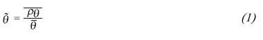
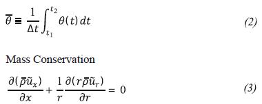
In this equation, the horizontal bar on the variables refers to the time average of these variables, which is shown in Equation 2.
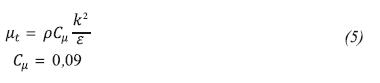
Energy Conservation
The turbulent viscosity is related to the turbulent kinetic energy (k) and the turbulent kinetic energy dissi-pation rate (ε) as follows:
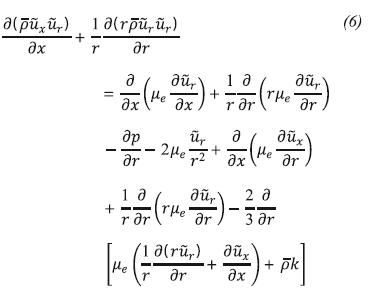
Momentum Conservation in the Direction r
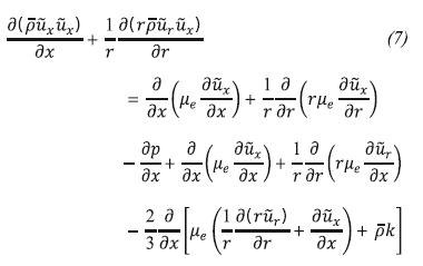
Momentum Conservation in the Direction x
Chemical Species Conservation
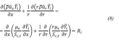
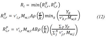
Ri is the production rate of specie i, which is calculated using the Finite rate/Eddy dissipation model which computes the Arrhenius reaction rate and a reaction rate based on the work of Magnussen and Hjertager (1976), taking as net reaction rate the smaller of both.
The production rate of specie i, is given by:
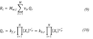
kf,r is the forward rate constant for reaction r that is calculated using the Arrhenius expression:

The rate of production of the chemical specie i calculated with the eddy dissipation model is:
Although multi-step reaction mechanisms may be used with the finite rate/eddy dissipation model, these likely produce incorrect solutions. This is due to multi-step chemical mechanisms based on Arrhenius rates, which differ for each reaction. In the eddy-dissipation model, every reaction has the same turbulent rate; therefore the model should be used only for one-step, or two-step global reactions (Fluent user's guide, 2006).
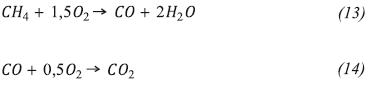
Reaction mechanism
It is used as a methane global reaction mechanism (Westbrook & Dryer, 1981) with two irreversible steps which are shown below.
Radiation Model
To calculate the source term in the energy equation (Sh) we use the P1 model (Siegel & Howell, 2002) because of its simplicity and good results obtained by:
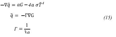
The absorption coefficient a is considered variable and it is calculated using a weighted sum of gray gases model (WSGGM).
k-ε Standard Turbulence Model
Since the turbulence viscosity (Equation 5) is in terms of two unknown variables, which are the turbulent kinetic energy and the turbulent kinetic energy dissipation rate, it requires two additional transport equations to find these two variables. The standard k-ε model developed by Launder and Spalding (1972) is used. This is a semi-empirical model based on model transport equations for the turbulence kinetic energy (k) and its dissipation rate (ε). The model transport equation for k is derived from the exact equation, while the model transport equation for ε was obtained using physical reasoning and shows some resemblance to its mathematically exact counterpart.
In the derivation of the standard k-ε model, the assumption is that the flow is fully turbulent, and the effects of molecular viscosity are negligible. Therefore this model is valid only for fully turbulent flows (Fluent user's guide, 2006).
Turbulent kinetic energy transport equation (k)
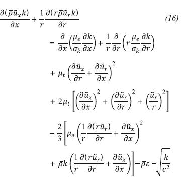
Turbulent kinetic energy dissipation rate transport equation (ε):
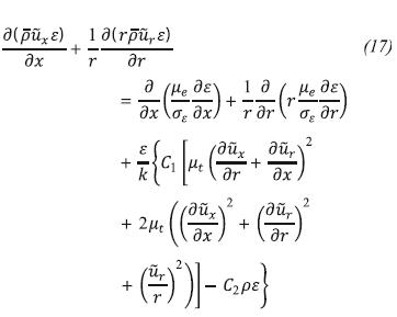
The symbols C1, C2, σk, σε are model constants and in this case the Fluent default values are used, which are recommended in the work of Launder and Sharma (1974).

These values have been determined from experiments with air and water for fundamental turbulent shear flows including homogeneous shear flows and deca-ying isotropic grid turbulence. They have been found to work fairly well for a wide range of wall bounded and free shear flows.
Numerical Method
To discretize all the variables, upwind second order schemes have been used, except for the pressure where the PRESTO scheme (Patankar, 1980) was used and momentum where upwind first order scheme was used. To consider the gas compressibility, the ideal gas law was used.
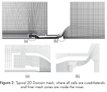
All 2D simulations have the same shape of the mesh, differing only in the openings of the regulators of pri- mary and secondary air as shown in Table 1. The meshes have approximately the same amount of cells (46 000 after two mesh adaptations). The areas needing increased mesh density are the mixer and the furnace dome. This happens because they have the highest gradients of speed, due to gas discharge, and of temperature, due to flame. Regarding the quality of the mesh, the higher aspect ratio is 7,6 and the equi angle skewness does not exceed 0,6. Figure 2 shows a typical mesh used in 2D axisymmetric simulations.
To determine if a simulation has converged, three different criterions have been used: first, the verification that residuals of the iterations are asymptotic. Then, a computed energy balance between inputs and outputs, which should be less than 5% of burner power. Finally, an average temperature and velocity in a line located in reaction zone, unchangeable despite iterations.
Three mesh adaptations have been done to each sin- gle simulation in order to outline the quantity of meshes necessary to obtain a mesh-independent solution. The adaptations were performed based on temperature and velocity gradients, determining that after around 45 000 cells, the solution is mesh independent in all simulations. This was concluded by comparing temperature profiles in a line located in the reaction zone with different cell quantities, and observing that there were no differences in these profi les, between successive cell quantities. Also, due to the operating conditions, the burner has a very turbulent flow. Therefore, in order to obtain good results with a standard k-ε model, the cells near the wall have been adapted to obtain a Y-plus (Y+ ) around 50 or less in all simulations./
Since the burner is a premixed burner, to ensure that the flame is generated in the burner head discharge and not inside the mixer, it is necessary to apply a high temperature (3 000K) region in the dome, before the iterations begin, which works like a spark plug to start chemical reactions in a desired region, consequently forming the flame.
Boundary Conditions
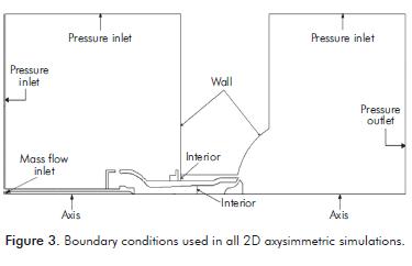
Figure 3 shows the boundary conditions used in all 2D-axysimmetric simulations. All pressure inlet condi- tions have a gauge pressure equal to zero, where air is used as fluid entering on these boundary conditions. As a result, the burner is simulated as discharging into the free atmosphere and not into a furnace. The walls are supposed to be adiabatic, so there is no heat transfer through these. Finally, the boundary conditions called interior conditions are used to take the profiles of velocity, temperature, turbu- lent kinetic energy, turbulent kinetic energy dissipation rate and methane, oxygen and nitrogen mass fraction. These are used as input conditions in the 3D simulation, which is done through a defi ned function by the Fluent user.
3. 2D-AXISYMMETRIC RESULTS
The results presented here correspond to those obtained in 2D simulations with different primary and secondary air regulator openings.
Burner Flow
Figure 4 shows the flow in the S8 burner simulation, observing the way it enters the primary and secondary air by the respective regulators.
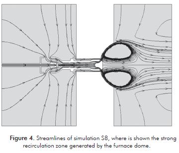
It also highlights the strong recirculation zone that is generated due to the dome in the furnace wall, which helps to provide stability of the flame, shortening it and preheating the air fuel premix.
Temperature Contours
Chemical reactions are produced between the exit of the burner head and the dome carved into the furnace wall, whose spherical shape contributes to stability of the flame and recirculation of the combustion products. In this way, the combustion efficiency is improved by preheating the premix discharged.
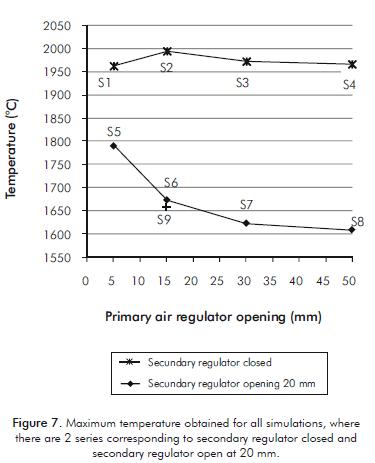
Figure 5 shows the temperature contours obtained when the primary air regulator is only opened. Figure 6 shows the temperature contours when the secondary air regulator is opened in 20 mm. In general, when the secondary air regulator is closed, the temperatures are higher and the flame tends to be more extended because there is no enough air to completely burn the fuel.
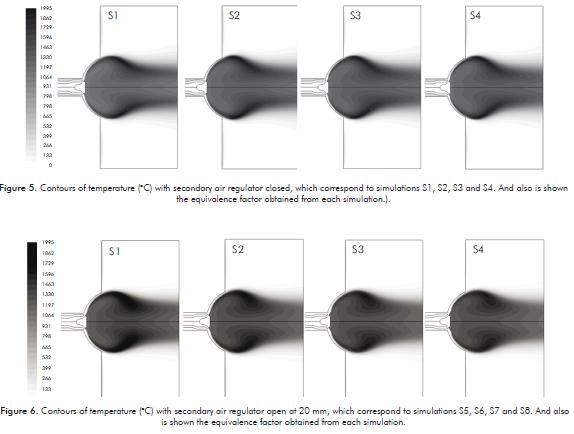
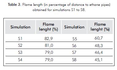
Figure 7 shows the maximum temperatures obtained in the simulations S1 to S9, observing that when the secondary air regulator is closed, the maximum temperature remains almost constant and close to the adiabatic flame value for methane, This occurs because the equivalence ratio always remains above 1 for all these simulations. Whereas when the secondary air regulator is opened in 20 mm, the maximum temperature tends to decrease as the opening of the primary air regulator increases. This happens because the amount of air is greater than the stoichiometric (except simulation S5), which has the effect of decreasing the temperature. This happens because part of the fuel energy is used to heat not reacting air.
Another important result that is derived from temperature contours is related with flame length, which in this work is defined as the maximum x-distance where some temperature contour is equal to 1 500°C. The results are presented in Table 3 for different simulations in a percent value, which is the relation respect to the distance of ethane pipes inside the furnace. This is useful because it allows seeing if the flame reaches the pipes, which in turn will reduce their lifespan. If this happens, the possibility of changing the burner design should be considered.
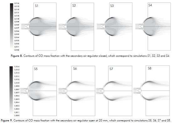
CO Contours
In Figure 8 and 9, the CO contours for simulations are presented. These have the secondary air regulator closed and opened in 20 mm respectively, where the amount of CO produced is quite large compared to when the secondary air regulator is opened. This happens because regardless of the openings of the primary air regulator, the air factor does not exceed the stoichiomaetric value. Therefore, there is not enough air to complete methane combustion.(Figure 10).
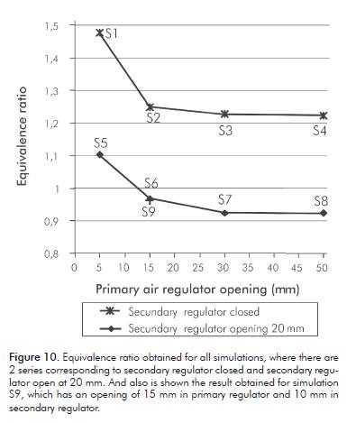
Equivalence Ratio
The equivalence ratio (f) is defined as the mass ratio of fuel-air ratio present during combustion divided by stoichiometric fuel-air ratio.
Where F is the mass of fuel, A is the mass of air and the suffix stoich stands for stoichiometric conditions.
Figure 10 shows the results obtained for the equivalence ratio with the secondary air regulator closed and opened in 20 m. It is observed that when the secondary air regulator is closed, the equivalence ratio is never lo-wer than the unit, and consequently there is air absence. If air is not added later, combustion remains incomplete. On the other hand, when the secondary air regulator is opened in 20 mm, and the primary air regulator has an opening larger than 15 mm, the equivalence ratio is lower than unity, reaching values of around 9% in air excess. Therefore, the amount of air amount is sufficient to complete combustion.
4. 3D SIMULATION
Given that in the 2D simulations the effect that divisions of the burner head have on the shape and characteristics of the flame has been neglected, we decided to take the profiles of some flow properties of a representative 2D simulation to serve as entry conditions into a 3D simulation. In this scenario, the flow from the burner head with the formation of the flame is simulated, in order to observe the differences with the corresponding 2D simulation.
To perform the 3D simulation, the following is used as input conditions: velocity profiles, turbulent kinetic energy (k), turbulent kinetic energy dissipation rate (ε), and density and concentration species (O2 , CH4) extracted from the S9 simulation. To use the profi les obtained from the 2D axisymmetric simulation as input conditions into the 3D simulation, a small user defi ned function (UDF) has been programmed in Fluent.
3D Mesh
The creation of the 3D mesh starts from the burner head. This mesh corresponds only to one quarter of the real burner due to symmetry, and includes the burner head, the furnace dome where the flame is formed and a part of discharge zone that is made of cylindrical shape (Figure11).
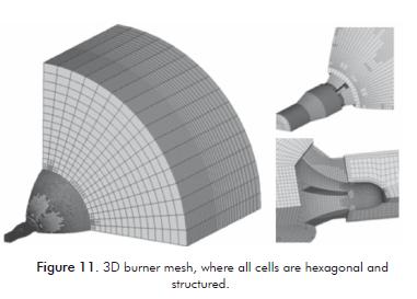
The original mesh has approximately 39 000 hexahedral cells, with an aspect ratio of 7,72 and an equi angle skewness maximum of 0,52. When performing the adaptation process in FLUENT, the mesh reaches -in the final simulation- a total of about 13 0000 cells.
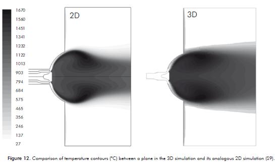
3D Results
Figure 12 is a comparison between the flame shape in a 2D simulation and a plane in a 3D simulation passing through the middle of a gas discharge channel. It can be observed that the basic shape of the flame and temperature profiles are preserved, but the flame in the 3D simulation is more robust than the corresponding 2D flame, being the latter more fl attened and elongated. This behavior was expected because the output section of the burner head was worked out in detail in the 3D simulation, obtaining more compact jets with greater penetrating power of the reactive mixture air-methane in the internal environment of the furnace.
To observe more clearly the flame shape, Figure 13 shows two iso surface temperature of 1 000°C and 1 300°C, on which the profiles of CO mass fraction are plotted. One of the main effects that the divisions located in the burner head on the flame shape have, is to deform the profi les, making them not completely axisymmetric, differing mainly from the results obtained in 2D simulation. In conclusion, the velocity, temperature and spe- cies profiles obtained with 2D and 3D simulations have differences in shape. Nevertheless, for practical aspects, the 2D simulation results show us a pretty good approxi- mation of the velocity, temperature and chemical species concentration (O2, CH4, CO, CO2) taking about 5 times less in computation time.
5. CONCLUSIONS
In this simulation work, the following aspects were concluded:
- Regarding the opening of the primary air regulator, it has no impact on equivalence ratio from around 30 mm, no matter the position of the secondary air regulator.
- When there is no secondary air entry, regardless of the primary air regulator opening, combustion air will always be lacking, indicating that the secondary air regulator plays an important role by providing remai-ning air to complete combustion.
- It is possible to obtain equivalence ratio lower than 1 (air excess), having the primary air regulator opened in values higher than 15 mm and maintaining the secon-dary air regulator open.
- The closure of the secondary air regulator has the fo-llowing consequences: increased production of CO, being always greater than the amount produced with the secondary regulator open, causing the combustion to be more inefficient; increasing flame temperature, since there is a lack of air and higher temperatures for methane are achieved with the absence of air near the stoichiometric (equivalence ratio greater than 1). Due to the absence of air in the combustion, the flame tends to be a bit more elongated than with the secondary air regulator opened, becoming more a diffusion flame.
- Although the shape of the flame differs from the 2D simulation respect to the 3D simulation, the latter takes into account the interaction of flow with the divisions in the burner head. To establish operating parameters, the 2D study is sufficient, since the contours of temperature, speed and other properties in the 3D simulation are similar with the results in 2D, being rather useful 3D simulation to observe more clearly the shape of the flame.
ACKNOWLEDGMENTS
The authors express their gratitude to Ecopetrol S.A. - Instituto Colombiano del Petróleo (ICP) and to Rosa Imelda Rueda for her collaboration in the development of this work.
REFERENCES
Arrieta, A. B., Cadavid, F. S. & Arrieta, A. A. (2011). Simulación numérica de hornos de combustión equipados con quemadores radiantes. Ingeniería y Universidad, 15 (1), 9-28. [ Links ]
Bidi, M., Hosseini, R. & Nobari, M. (2008). Numerical analysis of methane-air combustion considering radiation effect. Energy Conversion and Management, 49 (12), 3634-3647. [ Links ]
FLUENT version 6.3 User's guide (2006). Modeling species transport and finite-rate chemistry, Chapter 14. Fluent. [ Links ]
Herrmann, M. (2006). Numerical simulation of turbulent Bunsen flames with a lever set flamelet model. Combustion and Flame, 145: 357-375. [ Links ]
Jiang B., Liang H., Huang, G. & Li, X. (2006). Study on NOx Formation in CH4/Air Jet Combustion. Chinese J. of Chem. Eng., 14 (6), 723-728. [ Links ]
Launder, B. & Sharma, D. (1974). Application of the energy dissipation of turbulence to the calculation of flow near a spinning disc. Heat and Mass Transfer., 1 (2), 131-138. [ Links ]
Launder, B. & Spalding, D. (1972). Lectures in mathematical models of turbulence. London, UK: Academic press. 169. [ Links ]
Magnussen, B. & Hjertager, B. (1976). On mathematical models of turbulent combustion with special emphasis on soot formation and combustion. In 16th Symp.(Int'l) on Combustion. The Combustion Institute, Pittsburg, Pennsylvania. 719-729. [ Links ]
Patankar, S. V. (1980). Numerical heat transfer and fluid flow, Taylor and Francis. 118-120. [ Links ]
Roy, C. & Blottner, F. (2006). Review and assessment of turbulence models for hypersonic flows. Progress in Aerospace Sciences, 42 (7-8), 469-530. [ Links ]
Siegel, R. & Howell, J. (2002). Thermal radiation heat transfer, (4). New York: Taylor and Francis. [ Links ]
Westbrook, C. & Dryer, F. (1981). Simplified reaction mechanisms for the oxidation of hydrocarbon fuels in flames. Combustion Science and Technology, 27 (1-2), 31-43. [ Links ]
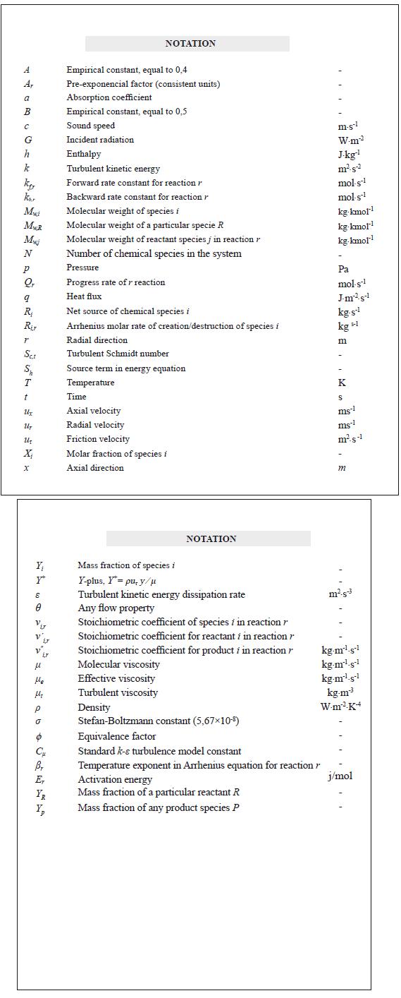
NOTATION