A PROPOSAL FOR REGULARIZED INVERSION FOR AN ILL-CONDITIONED DECONVOLUTION OPERATOR

PROPUESTA DE INVERSIÓN REGULARIZADA PARA UN OPERADOR DE DECONVOLUCIÓN MAL CONDICIONADO

Herling Gonzalez^1*, Sheryl Avendaño² and German Camacho¹

¹Ecopetrol S.A. - Instituto Colombiano del Petróleo (ICP), A.A. 4185 Bucaramanga, Santander, Colombia
²UTP Consultorias, Bucaramanga, Santander, Colombia

E-mail: herling.gonzalez@ecopetrol.com.co

(Received: Jun. 04, 2013; Accepted: Dec. 19, 2013)

*To whom correspondence should be addressed

ABSTRACT

From the inverse problem theory aspect, deconvolution can be understood as the linear inversion of an ill-posed and ill-conditioned problem. The ill-conditioned property of the deconvolution operator make the solution of inverse problem sensitive to errors in the data. Tikhonov regularization is the most commonly used method for stability and uniqueness of the solution. However, results from Tikhonov method do not provide sufficient quality when the noise in the data is strong. This work uses the conjugate gradient method applied to the Tikhonov deconvolution scheme, including a regularization parameter calculated iteratively and based on the improvement criterion of Morozov discrepancy applied on the objective function. Using seismic synthetic data and real stacked seismic data, we carried out a deconvolution process with regularization and without regularization based on a conjugated gradient algorithm. A comparison of results is also presented. Applying regularized deconvolution on synthetic data shows improved stability on the solution. Additionally, real post-stack seismic data shows a direct application for increasing the vertical resolution even with noisy data.

Keywords: Tikhonov regularization, Conjugated gradient, Theory inversion, Seismic processing.

RESUMEN

Desde el punto de vista de la teoría de problemas inversos, la deconvolución puede ser entendida como una inversión lineal de un problema mal-puesto y mal-condicionado. La característica del mal-condicionamiento del operador de deconvolución hace que la solución del problema inverso sea sensitiva a errores en los datos. La regularización de Tikhonov es el método más común empleado para estabilizar la solución y obtener su unicidad. Sin embargo, los resultados del método de Tikhonov no proveen calidad suficiente cuando el ruido en los datos es fuerte. Este trabajo hace uso del método del gradiente conjugado, basado en el esquema de Tikhonov aplicado a la deconvolución, cuyo parámetro de regularización es calculado iterativamente teniendo en cuenta el criterio de discrepancia de Morozov en la función objetivo. Haciendo uso de datos sísmicos sintéticos como datos reales apilados, se llevó a cabo el proceso de deconvolución con y sin regularización basada en el algoritmo del gradiente conjugado. Se llevó a cabo una comparación del esquema planteado. Aplicando la deconvolución regularizada en los datos sintéticos muestra una mejora en la estabilidad de la solución y los datos sísmicos post-apilados mostraron un incremento de la resolución vertical aun con ruido en los datos.

Palabras clave: Regularización de Tikhonov, Gradiente conjugado, Teoría de inversión, Procesamiento sísmico.

RESUMO

Desde o ponto de vista da teoria de problemas inversos, a deconvolução pode ser entendida como uma inversão linear de um problema mal posto e mal condicionado. A característica do mal condicionamento do operador de deconvolução faz que a solução do problema inverso seja sensitiva a erros nos dados. A regularização de Tikhonov é o método mais comum utilizado para estabilizar a solução e obter sua unicidade. Porém, os resultados do método de Tikhonov não fornecem qualidade suficiente quando o ruído nos dados é alto. Este trabalho faz uso do método do gradiente conjugado, baseado no esquema de Tikhonov aplicado à deconvolução, cujo parâmetro de regularização é calculado iterativamente tendo em conta o critério de discrepância de Morozov na função objetivo. Fazendo uso de dados sísmicos sintéticos como dados reais empilhados, foi realizado o processo de deconvolução com e sem regularização baseado no algoritmo do gradiente conjugado. Realizou-se uma comparação do esquema proposto. Aplicando a deconvolução regularizada nos dados sintéticos mostra uma melhoria na estabilidade da solução e os dados sísmicos pós-empilhados mostraram um aumento da resolução vertical mesmo com ruído nos dados.

Palavras-chave: Regularização de Tikhonov, Gradiente conjugado, Teoria de inversão, Processamento sísmico.

1. INTRODUCTION

Deconvolution is an inversion process that is co-mmonly used in many areas of science and engineering such as image and signal processing. In reflection seismic applications, deconvolution increases the vertical resolution. A basic model for a seismic trace is that it can be described by the convolution of a reflectivity series with a wavelet and added noise. Deconvolution results are generally considered as an approximation to the reflectivity series in a stratified medium, estimated from the reflected wavefield. There is extensive literature on the development of new inversion algorithms that improve deconvolution quality. Deconvolution quality in seismic data is assessed by its capacity to correctly predicting the position, amplitude and phase of the reflectivity series (Yilmaz, 1987; Zala, 1992; Leinbach, 1995). Deconvolution problems can have deterministic or non-deterministic approaches, depending on whether the wavelet is known or not (Wang, Wang & Perz, 2006). In this paper, we have assumed that the wavelet is known and band-limited, and have been estimated, for instance, from well log data or by statistical correlation of seismic data. The deconvolution process can be achieved by using regularization in the inversion (Karsli, Guney & Senkaya, 2012; Chen, Wang & Chen, 2012). By imposing an additional constraint on the estimated model, regularization can be implemented even if the convolution operates with insufficient data (Fomel, 2007) or when data contain high noise level (Hansen, 2010).

The solution to inverse problems commonly have stability issues and a multiplicity of solutions (Sen, 2006). From the mathematical standpoint, all inverse problems can be classified as well-posed or ill-posed. According to Hadamard (1923), an inverse problem is well-posed on the strict sense if:

1. There is a solution.
2. The solution is unique.
3. The solution is stable with respect to perturbations in the data.

Stability is related to the fact that minor changes introduced in the data of the problem generate minor variations in the solution. If any of the three conditions is not met, the problem is defined as ill-posed. Errors produced during measurement, as well as those introduced by numerical methods disassociate the extracted solution from the estimated information (Hansen, 2010; Montenegro, 2010). Techniques that enable recast from an ill-posed problem to a well-posed problem are also known as regularization. Deconvolution is an inverse problem, known for its sensitivity to noise in geophysical data processing (Van der Baan & Pham, 2008).

In this paper we propose an additional iterative calculation to estimate the regularization parameter e_i within the Tikhonov regularization scheme applied to the deconvolution of noisy data. This iterative calculation uses the bi-section and drying methods to find roots in the solution and the Morozov (1984) discrepancy criteria. We have also used concepts of deblurring theory on the convolution of seismic traces. The results of the regularized deconvolution method, presented here, show an improvement in the stability of the solution in the presence of noise, as well as a direct application for increasing the vertical resolution of stacked seismic data.

2. TIKHONOV REGULARIZATION

Tikhonov regularization suggests (for the inversion problem) adding a stabilizing matrix or function (Ti-khonov, 1963) such that:

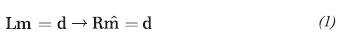
where L is the convolution operator, R is the regularized version of the operator, m is the physical model or series of reflectivity and is the approximate solution of the model, d is the response to the model m and d^ˆ are the data with noise from the seismic data. A regularized least-square solution l₂ of (1) is equivalent to minimizing the function

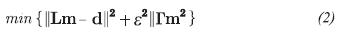
where ε is a parameter of regularization and Γ is the regularizing matrix (Fomel, 2007). This can be the identity I operator or a first order finite differences D matrix. Therefore, for the linear system with noise in (1), the best approximate solution can be obtained by minimizing the "functional smoothing" in (2) with an optimal value of ε (Tikhonov & Arsenin, 1977). D has a smoothing nature to ensure the linear variation of Lm around the proximity of m (Sen & Roy, 2003). In our case, the solution approximated by least squares of (2) is (Fomel, 2007):

This solution is regularized for a given value e accor-ding to the following expression (Hansen, 2010):

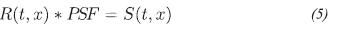
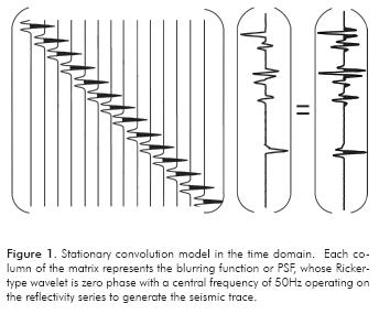
Following a convolution model for the seismic trace, we have assumed the reflectivity data as R(t) convoluted with a punctual blurring function called the Point Spread Function (PSF), which generates seismic data S(t). This function is equivalent to the seismic wavelet and is assumed to be constant and time inva-riant. PSF in image processing is a blurring function that lowers image resolution and, for our purposes, is one-dimensional.

Any pseudo-multidimensional array of traces, can be expressed as:

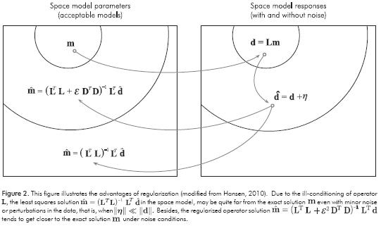
where variable t is the Two Way Time (TWT ) of the trace and variable x represents the horizontal coordinate (or offset) of traces. The above expression is analogous to our linear system Lm =d where L is the convolution matrix or function PSF, see Figure 2. By using elements ρi of matrix PSF with an odd magnitude 2r+1, we have a Toepliz matrix of the (n+2r) x (n) dimension, for this operator (Hansen, 2002):

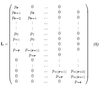
so we can carry out the deconvolution process to find in accordance with expression (3).

3. REGULARIZATION AND CONJUGATE GRADIENT

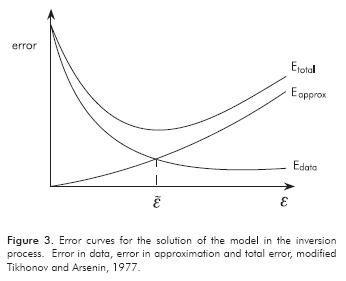
The effect of parameter e in the solution of Equation 14 is described as follows: When ε > 1, the regularization solution is stable. However, as tradeoff, the error of increases with respect to solution m. When ε < 1, the error of decreases, but regularization becomes unstable and sensitive to noise, leading to unwanted solutions (Tikhonov & Arsenin, 1977; Hansen, 2010), see Figure 2. Taking into account the error in the data, we can go further than Equation 1:

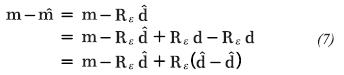
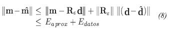
where . Taking into account the error in the approximation of the model and the error in the data, the error in the calculation of the model is:

The error in the data is expressed as the vector , that we call "tolerance". The magnitude of vector η is related iteratively with through the configurate gradient algorithm.

When To understand the effect of ε→ 0, we took in consideration the condition cond (L) of operator-matrix L

From this last expression, it can be proposed that there is a set of {εi} that optimize in a comprehensive manner the trade-off between error in the data and the error in approximation of the model (Figure 3).

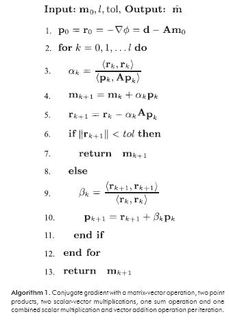
The technique chosen to minimize Equation 4 is the conjugate gradient technique, which consists of quadratically expressing linear relationship A m= d as:

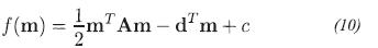
where A is a direct modeling operator with a defined positive square (Hestenes & Stiefel, 1952), (m, Am)= m^T (Am,m)>0, and symmetrical matrix A^T=A, here (,) represents the internal product. This quadratic vector equation is in terms of m whose gradient is equal to:

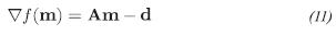
where the direction of maximum decrease is -∇ƒ=d-Am. The conjugate gradient method is a method of descent that begins to iterate in an initial model m₀ and continues in the direction of maximum descent of the paraboloid represented by quadratic function (10), resulting in a succession of models m_k that converge at a solution close to m.

By using the conjugate gradient method, we calculate a value of εi for any given εi, such that the residual is minimized. As we have outlined in Figure 4, for a given value of ε between 0<ε_i≤1 and an initial model m₀ (i.e. initial residual is r₀=d-Lm₀), decreases until it reaches a critical value. Further iterations {k} of conjugate gradient, increase the residual (see Figure 4).

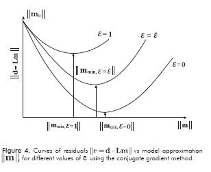
In Figure 4, notice that ε=0, is the solution of problem Lm=d, whose solution is unstable and sensitive to perturbations in data. Again, this is due to the ill-conditioned operator L (Shewchuk, 1994). In Figure 4, the curve with value ε=1, has a lower condition number for operator A=L^TL-D^TD, but the solution is not as close to the solution of the system. In the third curve in Figure 4 with optimal value ε=ε^∼, the solution is stable and close to m_ε-0, with a lower calculated residual value r. This behavior raises the question of how to choose this optimal parameter value.

To choose the optimal value ε=ε^∼ we have used the post-election strategy based on the discrepancy criteria (Morozov, 1984). This criteria establish that the norm of the difference between the observed data and the data generated by the regularized solution cannot be lower than the noise level δ:

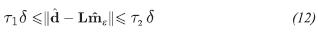
where (Bonesky, 2009). For our deconvolution problem we have taken . That means that the norm for the data generated by the regularized solution cannot be more accurate than the norm of the observed data (Engl, Hanke & Neubauer, 1996). In other words, the noise level δ should be proportional to ‌‌η‏‏, where , and proportional to . To estimate the relative noise level η in synthetic data, we have used normalization according to the following expression

Now, to estimate the relative noise level in seismic data, we have applied the following expression

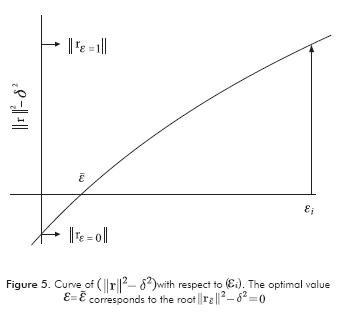
Now, we can assume that in order to obtain a proper , we have to find the values of the roots of equation (Montenegro, 2010). That is to say:

If the residual is larger than η and Equation 15 is positive, while for , the residual is smaller than and Equation 15 becomes negative. That suggest the iterative search , illustrated in Figure 5.

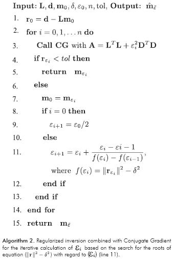
The following algorithm was developed to carry out the deconvolution process by regularization:

4. SYNTHETIC DATA

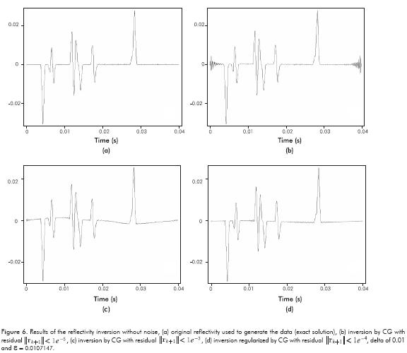
Tests with synthetic data enabled us to evaluate the response of the deconvolution process under the effects of noise in a controlled manner, as well as the results of the inversion strategy. We started with a simple case of deconvolution without noise. For the direct problem we use a zero phase Ricker wavelet with a central frequency of 50Hz (see Figure1) convoluted with a known reflectivity (see Figure 1 and 6a). The inversion result is presented in Figure 6b, which shows edge effects due to the sudden end of data at border (Gibbs oscillation). Changing the criteria of the residual value in the inversion process from 1x10^-5 to 1x10^-3, this edge effect is mitigated; however, the solution is not recovered (see Figure 6c). Then, using the regularization method suggested in Section 3 (Algorithm 2) and taking 1x10^-4 as the residual value, δ= 0.01 and an epsilon ε_i, of 0.0010715, we get the results displayed in Figure 6d. This illustrates in data the effect of trade-off between error in the data and error in approximation of the model. In a second numeric experiment, we added Gaussian noise to the data and the inversion was carried out in the same way as the previous experiment, i.e. taking a residual value of 1x10^-4, with and without regularization. The value of the Gaussian noise applied was lower than the residual of 1x10^-4. The effects of the noise on the inversion data are illustrated in Figures 7a and b.

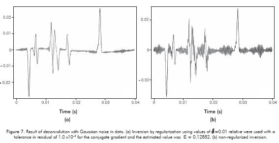
When noise is included in the data, the solution becomes unstable (Figure 7b) due to the ill-conditioning of operator L. Additionally, the CG method in the iterative process takes a larger number of steps for convergence (more than 300 iterative steps), sacrificing accuracy for stability. The difference in the results is due to the fact that the noise acts as a perturbation that is amplified in the iterative process due to the instability of the inversion. These results show the advantages of regularization when looking for stable solutions for an inversion problem in the presence of noise, as the deconvolution of real seismic data.

5. STACKED SEISMIC DATA

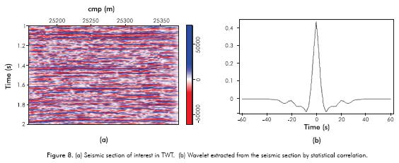
The method was applied on real seismic data extracted from a section of an area of interest. For the inversion-deconvolution process, a wavelet was statistically extracted in the target zone, where a preprocessing phase zero correction in seismic data was applied. The extraction of the wavelet is a common routine processin the oil industry for seismic characterization and seismic well calibration. The section analyzed was CMP 25160 to 25378 (218 meters) from 0 to 4 seconds in TWT. The target zone is between 1 and 2 seconds (see Figure 8a). The wavelet that was calculated is a Ricker (Figure 8b) estimated by statistical correlation.

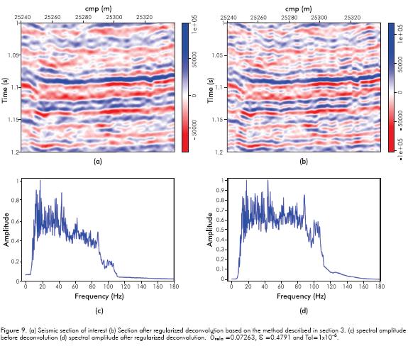
The deconvolution of this seismic section was carried out only with regularization (Figure 9) It is important to remember that the success of any inversion process with regularization is subject to the level of noise in data. If we have a seismic with poor image quality and high noise in the traces we cannot expect good results.

Different relative δ values were used between 0.1 and 0.01 for this regularized inversion in accordance with the discrepancy criteria and tolerance in the residual 1x10^-6. We have assumed that the rounding errors in calculations are less than the noise in the data. The inversion process applied is based on post-inversion as follows:

1. Estimating δ_rela with the CG method without regularization: The objective is to test the behavior of the error or residual with 100 or more ite-rations on the non-regularized solution, that is ε=0. If the residual does not vary or the deconvolution process declines in successive iterations for a given value of relative noise, it is taken as the limit to make the deconvolution invertible. Based on the Morozov criteria, nothing can be more accurate than the noise level. An exploration can be carried out with relative values of δ between 0.1 and 0.01 based on expression 14. If you know the uncertainty or standard deviation of the data you are working with, calculation δ_rela is direct and you would use Equation 13.

2. Defining tolerance and the initial value of ε_i: Considering the number of significant figures for precision and the adjustment of the minimum residual in the conjugate gradient algorithm (see Algorithm 2), the tolerance value should be consistent with the estimate of δ_rela in the previous step. To choose the (initial) e, it is important to consider the appropriate weighting between what you want to get and tolerance in the accuracy in the inversion. If we start with an ε=0, we are at the noise limit allowed and we get a poor quality image deconvolution. If we take a value of ε > 1, we are smoothing the result and moving away from the real solution. For practical proposals, it is a good idea to explore with initial values of ε≥1. This gives Expression 15 a root and leads to an optimal ε=ε^∼.

3. Assessing the result of the inversion process: Despite the application of the inversion theory and numerical implementation, the effectiveness of the regularized inversion process should be assessed with respect to the qualitative and quantitative analyses. A quantitative criterion independent from the vertical resolution that may be a comparison of the spectral amplitude is illustrated in Figures 9a and 9d. These spectra show that no abnormal frequencies were added and there was an improvement in the spectral amplitude to recover high frequencies. The above parameters change depending on these results. Therefore, it is post-inversion to preserve the balance between what you want and the tolerance in precision.

6. CONCLUSIONS

• This paper has shown how the inverse solution of an ill-conditioned operator (deconvolution) can be solved with a regularization model based on a conjugate gradient algorithm and stabilizing the solution to noise in data. We have illustrated the trade-off between error in the data and error in approximation of the model, that is, the balance between what you want and the tolerance allowed in the precision of solution.
• The optimal ε_i was found based on the Morozov discrepancy criteria, as a root of residual. The advantage of using the inversion model presented here was to find a satisfactory response for the deconvolution operator under the effect of Gaussian noise in data. An exact solution is not assumed in the inversion process obtained due to the level of noise in the data; the ill-conditioning of the deconvolution operator, the problems with errors in the floating point representation and the propagation of perturbations in the data. Numerical results have shown us how the solution can be stable under the influence of noise based on the Morozov discrepancy criteria, whose meaning suggests that nothing can be more accurate than the noise level. A successful application of the proposed regularization model was performed in real data.

ACKNOWLEDGEMENTS

The authors would like to thank Dr. Henry Lamos from Universidad Industrial de Santander for his invaluable discussion on the regularization model and the level of noise in data. They would also like to thank Dr. Sergey Fomel from University of Texas for his inspiration in regularized inverse problems and the development of the Madagascar application as a computer tool for the processing of the data presented herein. Finally, we thank Ecopetrol S.A. for its support in conducting this research.

REFERENCES

Bonesky, T. (2009). Morozov's discrepancy principle and Tikhonov-type functionals. Inverse Problems, 25(1), 1-11.         [ Links ]

Chen, Z., Wang, Y. & Chen, X. (2012). Gabor deconvolution using regularized smoothing. SEG Technical Program Expanded Abstracts, 2012: 1-5.         [ Links ]

Engl, H., Hanke, M. & Neubauer, A. (1996). Regularization of inverse problems. Dordrecht: Kluwer Academic Publishers.         [ Links ]

Fomel, S. (2007). Shaping regularization in geophysical-estimation problems. Geophysics, 72(2), R29-R36.         [ Links ]

Hadamard, J. (1923). Lectures on Cauchy's problem in linear differential equations. New Haven: Yale University Press.         [ Links ]

Hansen, C. (2002). Deconvolution and regularization with Toeplitz matrices. Numerical Algorithms, 29(4), 323-378.         [ Links ]

Hansen, C. (2010). Discrete inverse problems:Insight and Algorithms. Philadelphia: SIAM, Society for Industrial and Applied Mathematics.         [ Links ]

Hestenes, M. R. & Stiefel, E. L. (1952). Methods of conjugate gradients for solving linear systems. J. Research Nat. Bur. Standards, 49(6), 409-436.         [ Links ]

Karsli, H., Guney, R. & Senkaya, M. (2012). High resolution deconvolution by combining Fx filtering and cauchy regularization. 5th Saint Petersburg International Conference & Exhibition, EAGE.         [ Links ]

Leinbach, J. (1995). Wiener spiking deconvolution and minimum-phase wavelets: A tutorial. The Leading Edge, 14(3), 189-192.         [ Links ]

Montenegro, A. F. (2010). Regularización de problemas inversos e imágenes borrosas. Tesis de Maestría, Departamento de Geofísica, Universidad Nacional de Bogotá, Bogotá, Colombia, 87pp.         [ Links ]

Morozov, V. A. (1984). Methods for solving incorrectly posed problems. New York: Springer.         [ Links ]

Sen, M. & Roy, I. (2003). Computation of differential seismograms and iteration adaptive regularization in prestack waveform inversion. Geophysics, 68(6), 2026-2039.         [ Links ]

Sen, M. K. (2006). Seismic inversion. Austin: SPE.         [ Links ]

Shewchuk, R. J. (1994). An introduction to the Conjugate Gradient method without the agonizing pain. Report, School of Computer Science, Carnegie Mellon University, Pittsburgh, USA.         [ Links ]

Tikhonov, A. N. (1963). Solution of incorrectly formulated problems and the regularization method. Soviet Math. Dokl., 4: 1035-1038.         [ Links ]

Tikhonov, A. N. & Arsenin, V. Y. (1977). Solutions of ill-posed problems. Michigan: W. H. Winston.         [ Links ]

Van der Baan, M. & Pham, D. T. (2008). Robust wavelet estimation and blind deconvolution of noisy surface seismic. Geophysics, 73(5), 37-46.         [ Links ]

Wang, J., Wang, X. & Perz, M. (2006). Structure preserving regularization for sparse deconvolution. SEG Annual Meeting, New Orleans, Louisiana. Conference Paper 2006-2072.         [ Links ]

Yilmaz, Ö. (1987). Seismic data processing in geophysics. Tulsa: Society of Exploration Geophysicists.         [ Links ]

Zala, C. A. (1992). High-resolution inversion of ultrasonic traces. IEEE Transactions on Ultrasonics, 39(4), 438-463.         [ Links ]