Journal of oil, gas and alternative energy sources

A STATISTICAL ANALYSIS OF WIND SPEED DISTRIBUTION MODELS IN THE ABURRÁ VALLEY, COLOMBIA

ANÁLISIS ESTADÍSTICO DE MODELOS DE DISTRIBUCIÓN DE LA VELOCIDAD DEL VIENTO EN EL VALLE DE ABURRÁ, COLOMBIA

ANÁLISE ESTATÍSTICA DE MODELOS DE DISTRIBUIÇÃO DA VELOCIDADE DO VENTO NO VALLE DE ABURRÁ, COLÔMBIA

Paula-Andrea Amaya-Martínez¹, Andrés-Julián Saavedra-Montes¹ and Eliana-Isabel Arango-Zuluaga¹

¹ Universidad Nacional de Colombia, Medellín, Antioquia, Colombia

e-mail: ajsaaved@unal.edu.co

^* To whom correspondence should be addressed

How to cite: Amaya-Martínez, P. A., Saavedra-Montes, A. J. & Arango-Zuluaga, E. I. (2014). A statistical analysis of wind speed distribution models in the Aburrá Valley, Colombia. CT&F - Ciencia, Tecnología y Futuro, 5(5), 121-136.

(Received: Mar. 17, 2014; Accepted: Dec. 17, 2014)

ABSTRACT

The probability density functions, that model the wind speed behavior in five urban places and one rural of the Aburrá Valley in Antioquia, Colombia, are presented in this paper. The probability density functions are used to calculate the wind power density for each location, which are used to recommend several applications that could take advantage of such potential powers. Wind speeds are recorded at five monitoring stations located in the urban area of the valley and at one nearby rural station. Four probability density functions, namely, Weibull, Rayleigh, Gamma, and Lognormal, are used to represent the wind speed data histograms of each location and to select the probability density function that best fit the variability of the wind speed data. Also, four goodness of fit test are calculated. The wind power density is calculated with the probability density function that best represents the wind speed distribution to evaluate the wind power availability. The power densities reported for the five urban stations ranged from 1.38 to 4.54 W/m², and that reported for the rural station was 911.1 W/m². Taking into account the power density of each station, several applications are suggested.

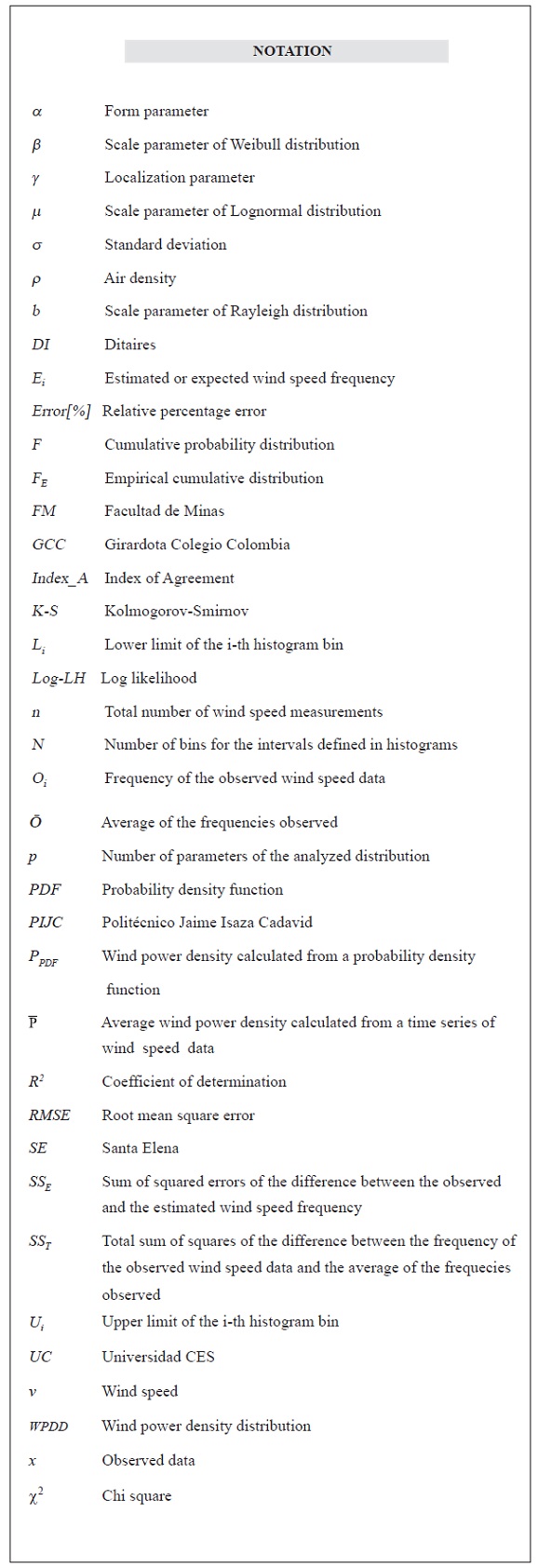
Keywords: Power density, Probability density function, Goodness of fit test, Wind speed.

RESUMEN

En este artículo se presentan las funciones de densidad de probabilidad que modelan el comportamiento de la velocidad del viento en cinco lugares urbanos y uno rural del Valle de Aburrá en Antioquia, Colombia. Las funciones de densidad de probabilidad son utilizadas para calcular la densidad de potencia en el viento para cada lugar, la cual es utilizada para recomendar varias aplicaciones que podrían aprovechar la potencia disponible. Las velocidades de viento son registradas en cinco estaciones de monitoreo ubicadas en el área urbana del valle y una estación rural cercana al Valle. Las cuatro funciones de densidad de probabilidad Weibull, Rayleigh, Gamma y Lognormal son usadas para representar los histogramas de los datos de velocidad del viento de cada ubicación y cuatro pruebas de bondad de ajuste son calculadas para seleccionar la función de densidad de probabilidad que mejor modela la variabilidad de los datos de velocidad del viento. Adicionalmente, la densidad de potencia en el viento es calculada con la función de densidad de probabilidad que mejor representa la distribución de velocidad del viento para evaluar la disponibilidad de potencia en el viento. Las densidades de potencia reportadas para las cinco estaciones urbanas están en el rango de 1.38 a 4.54W/m² y la densidad reportada para la estación rural es 911.1 W/m². Varias aplicaciones son sugeridas teniendo en cuenta la densidad de potencia de cada estación.

Palabras clave: Densidad de potencia, Función de densidad de probabilidad, Pruebas de bondad de ajuste, Velocidad del viento.

RESUMO

Neste artigo são apresentadas as funções de densidade de probabilidade que modelam o comportamento da velocidade do vento em cinco lugares urbanos e um rural do Vale de Aburrá, Antioquia, Colômbia. As funções de densidade de probabilidade são utilizadas para calcular a densidade de potência no vento para cada lugar, a qual é utilizada para recomendar várias aplicações que poderiam aproveitar a potência disponível. As velocidades de vento são registradas em cinco estações de monitoramento localizadas na área urbana do vale e uma estação rural próxima ao Vale. As quatro funções de densidade de probabilidade Weibull, Rayleigh, Gamma e Lognormal são usadas para representar os histogramas dos dados de velocidade do vento de cada localização e quatro provas de bondade de ajuste são calculadas para selecionar a função de densidade de probabilidade que melhor modela a variabilidade dos dados de velocidade do vento. Adicionalmente, a densidade de potência no vento é calculada com a função de densidade de probabilidade que melhor representa a distribuição de velocidade do vento para avaliar a disponibilidade de potência no vento. As densidades de potência registradas para as cinco estações urbanas estão na faixa de 1.38 a 4.54 W/m² e a densidade registrada para a estação rural é de 911,1 W/m². Várias aplicações são sugeridas considerando a densidade de potência de cada estação.

Palavras-chave: Densidade de potência, Função de densidade de probabilidade, Provas de bondade de ajuste, Velocidade do vento.

1. INTRODUCTION

The usage and application of renewable energies have increased significantly in recent years (Dincer, 2011; Fyrippis, Axaopoulos & Panayiotou, 2010; Hernández, Espinosa, Saldaña & Rivera, 2012). Wind energy is an important type of renewable energy that provides a clean and inexhaustible energy source (Li & Li, 2005a; Salameh & Nandu, 2010). The presence and behavior of wind are known through large-scale maps of wind at high altitudes around the world; however, less information is available regarding the presence and speed of wind in urban areas at low altitudes (Hernández et al., 2012; Li & Li, 2005b; Seguro & Lambert, 2000).

Local anemometric characteristics are used in wind statistical analysis. Among the available analytical tools, the Probability Density Function (PDF) stands out, which is used to assess the available wind energy at a given location and describes the variation of wind speed to optimize the design of wind energy conversion systems (Lo Brano, Orioli, Ciulla, & Culotta, 2011; Chang, 2011). This approach reduces the long time and resources that are associated with the processing of hourly wind speed information recorded during many years (Li & Li, 2005b). The most widely used PDFs correspond to the Weibull and Rayleigh distributions because they represent, with high precision, wind speed data from various geographical locations around the World (Acosta & Djokic, 2010; Akdag & Güler, 2010; Celik, 2004; Lo Brano et al., 2011; Safari, 2011; Safari & Gasore, 2010; Zhou, Erdem, Li & Shi, 2010). Other PDFs, such as the Gamma, Lognormal, Inverse Gaussian and Maximum Entropy Principle, have been used with positive results in some studies (Zhou et al., 2010; Li & Li, 2005a). In the Palermo urban area in Italy, the Weibull, Rayleigh, Lognormal, Gamma, Inverse Gaussian, Pearson type V and Burr PDFs, were the ones that best represented wind speed data (Lo Brano et al., 2011). Based on the references discussed above, it is clear that in urban areas there is wind potential which depends on the environment and building configurations. Although the Aburrá Valley is a tropical and deep valley where the wind speed is comparative smaller than other cities, it is necessary to characterize the wind speed using common PDFs to know the wind power and to take advantage of urban applications such as battery chargers and lighting.

Because there are several PDFs that could model the wind behavior in a specific place, it is necessary to select the PDF that best represents the wind speed. Zhou et al. (2010) used the chi square (χ²), coefficient of determination (R²), Root Mean Square Error (RMSE), log likelihood (Log-LH), Kolmogorov-Smirnov (K-S), and Index of Agreement (Index_A) goodness of fit tests to determine which PDFs showed the best adjustment to given locations avoiding biased results. More than one goodness of fit test is commonly used to guarantee the selection of the PDF that best models the wind speed in a specific place.

The assessment of available wind resources in a given location and time period is based on the calculated wind power density, which can be obtained by several methods. In Chang (2011) the wind power density is calculated from wind speed data as a time function. To obtain confident wind power density results, this method requires wind speed data measurements, which not always are available. Another is based on the wind PDF, which is used to calculate the Wind Power Density Distribution (WPDD). A comparison of the relative error between the WPDD obtained from the PDF and the WPDD obtained from wind data is considered when making a decision if a wind PDF is a good representation of the wind behavior (Li & Li, 2005a). The relative error between the power densities calculated by these two methods takes the power density calculated from the wind data as the reference value. Once a PDF is chosen to model the wind behavior of a specific place, it is necessary to calculate the wind power density and validate the result comparing it with the WPDD obtained from wind data.

The main objective of this work is to present the PDFs and their parameters, which model the wind speed behavior in five urban places and one rural of the Aburrá Valley in Antioquia, Colombia. Four goodness of fit test are used to select the PDF that best represent the wind speed behavior in each assessed location. Additionally, the wind power density for each location is calculated with the selected PDF and different applications are recommended to take advantage of such potential powers.

The rest of the paper is organized as follows: In Section 2 the methodology used to assess the wind resources in six locations of the Aburrá Valley is described. The results and their discussion are presented in Section 3. Finally, the conclusions are presented in Section 4.

2. METHODOLOGY

The methodology used to assess the wind resources in the five urban locations in the Aburrá Valley and the one nearby rural location is presented in this section. First, the study area and the monitoring station description are presented. Then, the four PDFs of the Weibull, Rayleigh, Lognormal and Gamma distribution used to fit the observed wind speed data are described. The four tests to evaluate the goodness of fit of each PDF are presented taking into account that they are the ones most widely used in previous works (Akpinar & Akpinar, 2007; Chang, 2011). Later in this section, the power density calculation using the PDF that best fits the histograms, and the average power density calculation using the observed wind data are described. The later method is used as a reference to validate if the selected PDF represents the wind behavior in the specific location.

Study Area and Monitoring Stations

The study was conducted in five urban locations within the Aburrá Valley and in one rural location outside but close to the valley, as shown in Figure 1. The Aburrá Valley, a natural basin of the Medellin River, is located in the central southern part of the Antioquia province in Colombia. The valley has an irregular and steep topography with altitudes ranging from 1300 m to 2800 m above sea level. The lower, flat part of this narrow valley has a maximum width of 10 km from east to west and a length of 70 km from south to north.

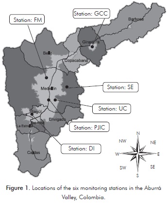
The names of the locations of the five urban monitoring stations are: Facultad de Minas (FM), Girardota Colegio Colombia (GCC), Politécnico Jaime Isaza Cadavid (PJIC), Universidad CES (UC), and Ditaires (DI). The rural station is called Santa Elena (SE). The anemometer at FM monitoring station is located 4 m above the ground. The station is influenced by high vehicular traffic. The distance from the station to the border road is 3 m and the road width is 12 m. The local environment of the station is residential, university and multiple activities. The PJIC station is located in a residential and multiple activities environment; and is influenced by high vehicular traffic. The distance from the station to the border road is 5 m and the road width is 7 m. The anemometer is located 6 m above the ground.

The GCC monitoring station is fixed and is located in a suburban area i.e. big green areas are mixed with built areas. The station is indirectly influenced by the traffic. The distance from the station to the border road is 4 m, the road width is 5 m, and the anemometer is 10 m above the ground. The DI monitoring station is fixed and is located in an industrial area; also the area is characterized as mandatory social use. There is not significant influence of vehicular traffic or tall buildings. The anemometer is 4 m above the ground. SE monitoring station is located in a rural area with a very small residential index and basically there is no building or roads affecting the station.

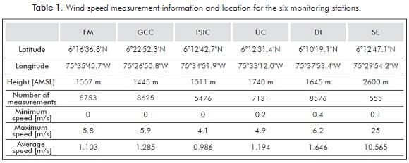
In all stations, the sampling time used was 60 minutes; this sampling time has been commonly used to record urban wind data in previous studies (Acosta & Djokic, 2010; Georgakis & Santamouris, 2008; Li, Wang, & Yuan, 2010; Lo Brano et al., 2011; Zhou et al., 2010). The wind data from urban areas were provided by the Air Quality Laboratory (CALAIRE) at Universidad Nacional de Colombia, and correspond to one year. The number of measurements and the minimum, maximum and average wind speeds for each station are summarized in Table 1. Also, the latitude, longitude and height of each station are provided. In certain cases, the number of measurements was lower than it should have been as a result of data loss during certain time periods.

Probability Density Functions (PDFs)

PDFs are mathematical functions that characterize the probable behavior of a data set. This data set can correspond to the behavior of a random variable that is continuous in time. Since wind speed is random variable, it is appropriate to describe those using PDFs. The Weibull, Rayleigh, Lognormal and Gamma PDFs have been used in many studies to evaluate the installation of wind turbines in a given location or to calculate the available wind resources (Acosta & Djokic, 2010; Fyrippis et al., 2010; Li & Li, 2005a; Lo Brano et al., 2011; Safari, 2011; Zhou et al., 2010).

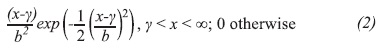
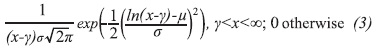
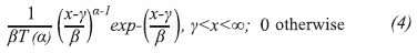
In this study, the maximum likelihood method was used to calculate the Weibull, Rayleigh, Lognormal and Gamma PDF parameters that maximize the probability of the recorded wind speed data. The maximum likelihood method is considered to be a precise and robust method (Lo Brano et al., 2011; Seguro & Lambert, 2000), and it is also the most appropriate computational method for the analysis of wind energy when the Weibull distribution parameters are estimated based on the wind speed data series (Seguro & Lambert, 2000; Zhou et al., 2010). The PDF parameters were calculated using the maximum likelihood method from the Statistical Analysis Software SAS^®. Weibull, Rayleigh, Lognormal and Gamma PDF definitions are given by Equation 1, 2, 3 and 4 respectively.

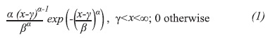
In Equation 1, 2, 3 and 4, x represents the observed data. The Weibull distribution has three parameters: the form parameter α, the scale parameter β, and the localization parameter γ. The family of curves that can be generated from the Weibull PDF using different parameters results in a good fit to the measured wind speed data because of the flexibility of the parameters and the capability of the function to adjust both exponential and normal shapes (Chang, 2011; Zhou et al., 2010).

The Rayleigh distribution is a special case of the Weibull distribution and is used frequently in the literature to fit wind PDFs (Lo Brano et al., 2011). One advantage of the Rayleigh distribution is that the PDF and the cumulative distribution function (F) are obtained from the average wind speed. In this PDF, the form parameter α is equal to 2 and the parameter β is equal to √2 times the b parameter from the Rayleigh distribution (Acosta & Djokic, 2010; Zhou et al., 2010).

The Lognormal distribution is used to fit wind speed variations and to generate frequency distributions of wind speed for a given time interval (Li & Li, 2005b; Lo Brano et al., 2011; Zhou et al., 2010). It is a probability distribution of a random variable whose logarithm has a normal distribution. The parameters of the PDF include the scale parameter μ, the standard deviation σ, and the localization parameter γ.

The first statistical studies of wind speed were performed approximately 60 years ago, and these studies considered wind speed to be a discrete random variable, and modeled it using a Gamma distribution. The generalized Gamma distribution is appropriate for describing the surface wind speed distribution in most of Europe (Lo Brano et al., 2011). This distribution represents the sum of exponential functions distributed as random variables, and its PDF includes the form parameter α, the scale parameter β and the localization parameter γ.

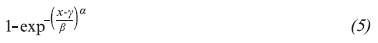
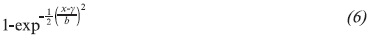
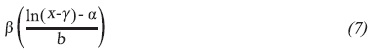
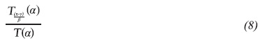
The cumulative PDFs of the Weibull, Rayleigh, Lognormal and Gamma distributions are given by Equations 5, 6, 7 and 8 respectively. These cumulative PDFs are used to calculate the goodness of fit test described in next subsection. The observed data are represented by x.

Goodness of Fit Tests

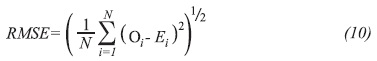
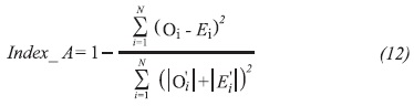
To evaluate the goodness of fit of the chosen distributions to the wind speed histograms, four tests were selected based on a literature review. The most commonly used tests are the R², RMSE, K-S and Index_A. The definitions of the four tests are presented in Equations 9, 10, 11 and 12 respectively (Li & Li, 2005a; Lo Brano et al., 2011; Ramírez & Carta, 2005; Zhou et al., 2010). R², RMSE and K-S tests have been used extensively to compare the statistical distributions obtained in wind speed modeling studies. The Index_A test has been applied in the analysis of statistical distributions to predict air contaminants and wind erosion.

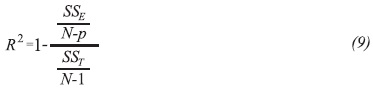
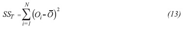
Coefficient of Determination (R²) Test

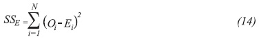
R² measures the degree of the linear relationship between the expected and the observed wind speed frequency values. N represents the number of bins for the intervals defined in the histogram and p is the number of parameters of the analyzed distribution. The total sum of squares SS_T of the difference between the frequency of the observed wind speed data (O_i), -which is the sum of the number of wind speed data that are included in the i-th histogram bin-, and the average of the frequencies observed () is given by Equation 13. The sum of squared errors SS_E of the difference between the observed and the estimated wind speed frequency is given by Equation 14. The estimated or expected wind speed frequency (E_i) is given by Equation 15, where F represents the cumulative probability distribution function evaluated at the upper (U_i) and lower (L_i) limits of the i-th histogram bin. These upper and lower limits correspond to the largest and smallest values of the wind speed for the bin analyzed. n is the total number of wind speed measurements. When the R² value is closer to 1, the fit of the data to the distribution used is better.

Root Mean Square Error (RMSE) Test

This test calculates the RMSE between the observed wind speed frequency O_i and the estimated wind speed frequency E_i. The result of the test may differ by several orders of magnitude, depending on whether the RMSE is calculated using the frequencies, the probability densities or the estimated wind speed probabilities. The RMSE value is larger when it is calculated with the frequencies than when it is calculated with the probability densities or the probabilities. When the RMSE of a PDF is closer to zero, the fit between the observed values and the values expected from the PDF is better. When the RMSE values for several PDFs are compared, it is necessary that these values are calculated using the same variable, i.e. frequency, probability density or probability to make a fair comparison.

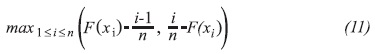
Kolmogorov-Smirnov (K-S) Test

This test is based on the maximum difference between the hypothetical and the empirical cumulative distributions (F_E). The empirical cumulative probability distribution function is defined by Equation 16:

Where E(i) is the number of points smaller than x_i, with x_i values sorted from smallest to largest. F_E is a step function that increases by 1/n at the value of each sorted data point. The null hypothesis in the K-S test is that the data follows a specific distribution. If the result of the test is lower than a critical value, the fit to the distribution is considered to be good. The K-S test was originally presented as a goodness of fit test by Massey Jr (1951) together with a critical value table.

Index of Agreement (Index_A) Test

Index_A, as shown by the definition in Equation 12, is the difference between the number 1 and the quotient of the sum of squares of the differences between the observed and the expected frequencies, and the sum of squares of the absolute values of the differences between the observed frequency values and their average -as given in Equation 17-, and the absolute values of the differences between the expected frequency values and their average -as given in Equation 18-. The possible values of Index_A range from 0 to 1. A value that is closer to 1 indicates a better fit of the PDF to the observed data histogram.

Wind Power Density

Wind power density is calculated to assess the availability of wind resources in a given location (Li & Li, 2005b). Wind power density is proportional to the cube of wind speed and for a selected PDF(v) can be calculated as shown in Equation 19 (Akpinar & Akpinar, 2007; Li & Li, 2005a; Chang, 2011):

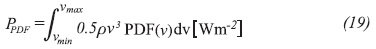
Where v_min and v_max correspond to the minimum and maximum wind speed data, respectively, which were used to obtain the parameters of the PDF. ρ represents the air density in kg.m^-3 and v represents the wind speed in m.s^-1.

When a time series of wind speed data is available, an average wind power density () can be calculated by Equation 20, which uses the average air density value and the cube of the average wind speed (Carta & Ramírez, 2007; Johnson, 1985; Chang, 2011):

Air density can be calculated from the equation CIPM-2007 approved by the International Committee for Weights and Measures (Picard, Davis, Gläser & Fujii, 2008).

3. RESULTS AND DISCUSSION

Comparisons Between the Distribution Functions and the Observed Data

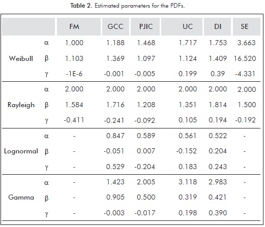
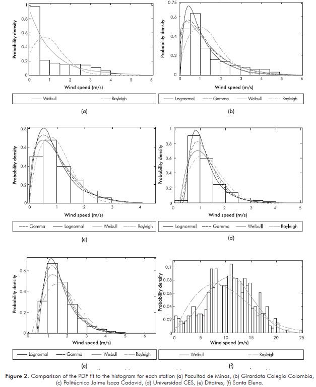
The values of the form α, scale β and localization γ parameters for each distribution and each station are presented in Table 2. The three parameters of Weibull and Rayleigh distributions were estimated for the five stations in the Aburrá Valley; however, the wind speed behavior for FM and SE stations was not described by the PDFs of Lognormal and Gamma distributions. For the latter two distributions, no reasonable PDF parameters could be found. The comparisons between the wind speed histograms and the PDFs of the distributions used to fit them are presented in Figure 2.

Each of the six wind distribution was represented by two or more PDFs. Goodness of fit tests, as defined in Equations 9-12, were performed to select the PDF of the distribution that best represented the behavior of the wind speed data for each location. The four goodness of fit test conducted to compare each PDF with the corresponding histogram are presented in Table 3. For each station, the distributions were sorted according to the coefficient of determination R². A value closer to 1 for this test indicates a distribution with a PDF that better fits the wind speed data. The calculated value of RMSE coincides with the value of R² because for each station the smallest RMSE value corresponds to the R² value closest to 1. The RMSEs were calculated using values of the observed and estimated frequencies as defined in Equation 10. The RMSE values obtained are larger than those obtained in similar studies (Akpinar & Akpinar, 2007; Li & Li, 2005b; Safari, 2011; Chang, 2011) because frequencies, rather than probabilities or probability densities, were used for the RMSE calculation.

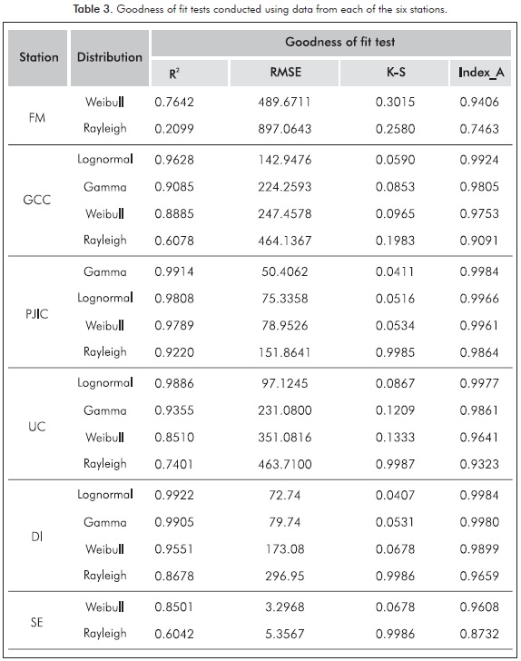
None of the results from the K-S test was less than the corresponding critical value from the Kolmogorov table. Therefore, the hypothesis that the distribution was a good fit to the observed data was not accepted; however, the trend of the K-S test results was consistent with those of the RMSE and R² tests. The Index_A test result equals 1 when the PDF of a given distribution represents the observed data exactly. The results from the Index_A test were in the same order as those from the R² test. For each station, there was at least one distribution that had an Index_A value greater than 0.99, which indicates a good fit of the data with the analyzed distribution. The results in Figure 2 are analyzed below for each location.

Facultad de Minas (FM)

The station at FM sampled data every hour. This station was characterized by low average speed 1.1034 m/s. The comparison of the observed data with the PDF used is presented in Figure 2a. The Weibull distribution best fit the behavior of the wind speeds for this station. However, the PDF has an exponential shape because the form parameter α was equal to 1. It should be taken into account that Weibull function does not represent all wind natural distributions, e.g. wind distributions with significance low winds, which are represented as cero wind speed in the Weibull function. Because in FM low wind speeds are predominant, Weibull function does not represent the wind distribution in that place.

Girardota Colegio Colombia (GCC)

This station had an average wind speed of 1.2854 m/s. The Lognormal distribution fit the wind speed behavior for this station best. The histogram of the observed data presented a single peak; therefore, the goodness of fit test calculated for the Lognormal distribution was better than the test calculated for the Weibull distribution. Figure 2b shows the comparison of the four distributions and the histogram of the observed data for GCC.

Politécnico Jaime Isaza Cadavid (PJIC)

The results of the goodness of fit tests in Table 3 show that the distribution that most closely fit the wind speed data recorded at this station was the Gamma distribution followed by the Lognormal and Weibull distributions. The comparisons between the PDFs and the histogram of the observed data for PJIC are presented in Figure 2c.

Universidad CES (UC) and Ditaires (DI)

The observed data for wind speed distributions at these two stations were similar, as shown in Figure 2d and Figure 2e. For both stations, the Lognormal distribution best fit the observed data followed by the Gamma, Weibull and Rayleigh distributions.

Santa Elena (SE)

This station was located in a rural sector close to the Aburrá Valley and had the highest elevation of the six monitoring stations. This difference is reflected in Table 1 by the fact that the average wind speed recorded at Santa Elena station was at least 6.4 times greater than that recorded at the Ditaires urban station with the highest average wind speed. The wind speed distribution at SE was fit only by the Weibull and Rayleigh distributions. Weibull was the distribution that best fit the data according to the results shown in Table 3. The comparisons between the observed data for SE and the distributions that best fit them are shown in Figure 2f.

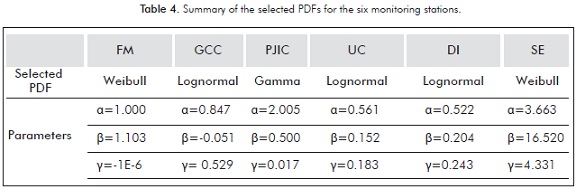
In Table 4 the selected PDFs, and their parameters, for the assessed places are presented. In order to know the specific place that is represented by the selected distribution, the latitude and longitude is provided. Once a distribution is selected, and its parameters estimated for a specific place, the wind power density can be calculated. However, to recommend a wind turbine installation place -and taking into account some goodness of fit test were no close to acceptable values (e.g. the R² for FM)-, it is necessary to confirm the PDF representation through the comparison between the wind power density calculated with PDF and with a time series of wind speed data.

Assessment of the Wind Power at the Six Monitoring Stations

The wind power at the six monitoring stations was assessed through the calculation of their power density by two methods at each location. In the first method the power density was calculated using Equation 20 and the wind speed data set recorded during a period of approximately one year. Figure 3 illustrates the wind behavior in the Aburrá Valley based on a series of wind speed data recorded at the PJIC station during four weeks. Table 5 presents the power density values [Wm^-2] calculated by Equation 20 for all stations. These values are used as references values to validate the wind power density calculated from the PDFs selected in Table 4.

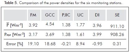
In the second method, the power density P_PDF [Wm^-2] is calculated using Equation 19 and the maximum and minimum wind speed values at the evaluated station. The wind power densities are given in Table 5. The relative percentage error between the power densities in a given location was calculated using Equation 21. The relative error is useful in order to know if the selected PDF is enough representation of the wind behavior in the specific place. For example, for GCC location: the R² (0.9628) and the Index_A (0.9924) report values near to one, which create the false idea that Lognormal distribution is enough representation for the assessed place. However, the relative error 18.68% indicates that other distribution should be evaluated to obtain a better representation of the wind behavior in GCC location.

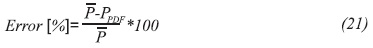
Table 5 shows that wind power densities calculated from the PDF for the PJIC, UC, DI and SE stations have relative errors less than 9%. The Lognormal distribution best fit the data for two of those stations. The power densities for FM and GCC stations have 19.1% and 18.68% relative errors respectively. The latter two error values suggest that different PDF should be adjusted for FM and GCC, in order to avoid over or under estimation of the wind energy in those places.

The five urban stations in the Aburrá Valley reported average power densities between 1.38 and 4.54 W/m², and the one rural station reported a value of 911.1 W/m². In agreement with the commercially international system of classification by Elliott and Schwartz (1993), the urban locations correspond to the wind power class 1, since the density value is lower than 100 W/m². Therefore, the five urban locations present wind characteristics that are not suitable to grid connected big scale applications. The power density levels reported in the urban locations are appropriate to electrical and mechanical applications that are not connected to the power grid, e.g. battery charging and water pumping.

Santa Elena location corresponds to the wind power class 7. It is generally accepted that wind power class 4 and higher types are suitable to big scale electricity generation using wind turbine modern technology, since the high power wind generators -in combination with a high wind resource- are competitive in cost in contrast with other electric power sources.

4. CONCLUSIONS

• In order to evaluate the available wind power in five urban places and one rural of the Aburrá Valley in Antioquia, Colombia, this paper has presented the PDFs and their parameters, which together, model the wind speed behavior in those locations. The PDFs were used to calculate the wind power density for each location, which are used to recommend several applications that could take advantage of such potential powers. The observed wind behavior is represented by the Weibull PDF at two of the locations, by the Lognormal PDF at three locations and by the Gamma PDF at one location. The power densities calculated with the functions that best fit the wind histograms have the lowest relative error with respect to the power densities calculated from the observed data. From the results of the goodness of fit tests and the comparison of the wind power densities, it is concluded that the wind behaviors of PJIC, UC, DI and SE are represented by the distributions selected in this work. Because calm wind is predominant in FM, none of the proposed PDF is a close representation. Therefore, different PDF functions are needed to represent the wind speed behavior in FM.


• The average power densities obtained are between 1.38 and 4.54 W/m² for urban locations and 911.1 W/m² for the rural one. The urban locations are suitable for electric and mechanical applications such as battery charging and water pumping. For Santa Elena, wind turbines could be installed to convert the available wind power. Also, those turbines can be connected to the power grid. Finally, this paper opens several work lines. One of them is the necessity to monitoring the wind speed in several cities of Colombia in order to know its wind potential and take advantage of it.

ACKNOWLEDGEMENTS

The authors acknowledge the Air Quality Laboratory at Universidad Nacional de Colombia for providing the wind speed data, and the Departamento Administrativo de Ciencia Tecnología e Innovación COLCIENCIAS for the doctoral scholarship 095-2005. This study was supported by the research project MICRO-RED 18687, which was financed by Universidad Nacional de Colombia.

REFERENCES

Acosta, J. L. & Djokic, S. Z. (2010). Assessment of renewable wind resources in UK urban areas. 15th IEEE Mediterranean Electrotechnical Conference, Malta.         [ Links ]

Akdag, S. A. & Güler, Ö. (2010). Evaluation of wind energy investment interest and electricity generation cost analysis for Turkey. Appl. Energy, 87(8), 2574-2580.         [ Links ]

Akpinar, S. A. & Akpinar, E. K. (2007). Wind energy analysis based on Maximum Entropy Principle (MEP)-type distribution function. Energy Convers. Manag., 48(4), 1140-1149.         [ Links ]

Carta, J. A. & Ramírez, P. (2007). Use of finite mixture distribution models in the analysis of wind energy in the Canarian Archipelago. Energy Convers. Manag., 48(1), 281-291.         [ Links ]

Celik, A. N. (2004). A statistical analysis of wind power density based on the Weibull and Rayleigh models at the southern region of Turkey. Renew. Energy, 29(4), 593-604.         [ Links ]

Chang, T. P. (2011). Estimation of wind energy potential using different probability density functions. Appl. Energy, 88(5), 1848-1856.         [ Links ]

Dincer, F. (2011). The analysis on wind energy electricity generation status, potential and policies in the world. Renew. Sustain. Energy Rev., 15(9), 5135-5142.         [ Links ]

Elliott, D. L. & Schwartz, M. N. (1993). Wind energy potential in the United States. International Academy of Science Project Energy, Kansas City, USA.         [ Links ]

Fyrippis, I., Axaopoulos, P. J. & Panayiotou, G. (2010). Wind energy potential assessment in Naxos Island, Greece. Appl. Energy, 87(2), 577-586.         [ Links ]

Georgakis, C. & Santamouris, M. (2008). On the estimation of wind speed in urban canyons for ventilation purposes-Part 1: Coupling between the undisturbed wind speed and the canyon wind. Build. Environ., 43(8), 1404-1410.         [ Links ]

Hernández, Q., Espinosa, F., Saldaña, R. & Rivera, C. (2012). Evaluación del potencial eólico para la generación de energía eléctrica en el estado de Veracruz, México. Dyna, 171: 215-221.         [ Links ]

Johnson, G. L. (1985). Wind energy systems. Englewood Cliffs: Prentice-Hall.         [ Links ]

Li, D., Wang, S. & Yuan, P. (2010). A review of micro wind turbines in the built environment. Power and Energy Engineering Conference (APPEEC), Chengdu, Asia.         [ Links ]

Li, M. & Li, X. (2005a). Investigation of wind characteristics and assessment of wind energy potential for Waterloo region, Canada. Energy Convers. Manag., 46(18), 3014-3033.         [ Links ]

Li, M. & Li, X. (2005b). MEP-type distribution function: a better alternative to Weibull function for wind speed distributions. Renew. Energy, 30(8), 1221-1240.         [ Links ]

Lo Brano, V., Orioli, A., Ciulla, G. & Culotta, S. (2011). Quality of wind speed fitting distributions for the urban area of Palermo, Italy. Renew. Energy, 36(3), 1026-1039.         [ Links ]

Massey, Jr, F. J. (1951). The Kolmogorov-Smirnov test for goodness of fit. J. Amer. Statis. Assoc., 46(253), 68-78.         [ Links ]

Picard, A., Davis, R., Gläser, M., & Fujii, K. (2008). Revised formula for the density of moist air (CIPM-2007). Metrologia, 45(2), 149-155.         [ Links ]

Ramírez, P., & Carta, J. A. (2005). Influence of the data sampling interval in the estimation of the parameters of the Weibull wind speed probability density distribution: a case study. Energy Convers. Manag., 46(15-16), 2419-2438.         [ Links ]

Safari, B. (2011). Modeling wind speed and wind power distributions in Rwanda. Renew. Sustain. Energy Rev., 15(2), 925-935.         [ Links ]

Safari, B. & Gasore, J. (2010). A statistical investigation of wind characteristics and wind energy potential based on the Weibull and Rayleigh models in Rwanda. Renew. Energy, 35(12), 2874-2880.         [ Links ]

Salameh, Z. & Nandu, C. V. (2010). Overview of building integrated wind energy conversion systems. IEEE Power and Energy Society General Meeting, Minneapolis, USA.         [ Links ]

Seguro, J. & Lambert, T. (2000). Modern estimation of the parameters of the Weibull wind speed distribution for wind energy analysis. J. Wind Eng. Ind. Aerodyn., 85(1), 75-84.         [ Links ]

Zhou, J., Erdem, E., Li, G., & Shi, J. (2010). Comprehensive evaluation of wind speed distribution models: Acase study for North Dakota sites. Energy Convers. Manag., 51(7), 1449-1458.         [ Links ]

AUTHORS

Paula-Andrea Amaya-Martínez
Affiliation: Universidad Nacional de Colombia
Industrial Engineering, Universidad Nacional de Colombia
e-mail: paamayam@unal.edu.co

Andrés-Julián Saavedra-Montes
Affiliation: Universidad Nacional de Colombia
Electrical Engineering, Universidad del Valle
M. Sc. in Systems Power Generation, Universidad del Valle
Ph. D. in Electrical Engineering, Universidad del Valle
e-mail: ajsaaved@unal.edu.co

Eliana-Isabel Arango-Zuluaga
Affiliation: Universidad Nacional de Colombia
Electronic Engineering, Universidad de Antioquia
Ph. D. in Electronic Engineering, Universitat Rovira I Virgili
e-mail: eiarangoz@unal.edu.co