


 English (pdf)
 Article in xml format
 Article references
 Send this article by e-mail
 Cited by SciELO
  Cited by Google
  Similars in
SciELO
Similars in
SciELO  Similars in Google
 Permalink
1. INTRODUCTION
Spectral Inversion has been used to highlight subsurface images with thin layers with thicknesses below one quarter of a wavelength (Castaño, Ojeda & Montes, 2011), and the reason is that a reliable estimate of layer thicknesses during exploration helps delineate prospects even in absence of well information. Consequently, consequently, the spectral inversion allows to estimate hydrocarbon reserves with more accuracy and better plan the drilling of production wells. Vertical resolution is key to extract a detailed stratigraphy that may differentiate two very close seismic events associated with geological facies, which is significant because major hydrocarbon reservoirs have been found in very thin layers which are below seismic resolution. Variations in wave amplitude and phase, caused by layers of different thicknesses, jointly with interference patterns, allow the extraction of stratigraphic details such as thicknesses and lateral continuity (Partyka, 2005). Now, as it is unlikely for a lithological unit to have the same coefficients at its top and its base, the relevant pair of reflection coefficients r1 and r2 may be decomposed into an even part (r1+ r2) 2 / and an odd part (r1- r2) 2 / (Castagna, 2004; Chopra, Castagna & Portniaguine, 2006). This results in the Spectral Inversion (Puryear & Castagna, 2008) that transforms the amplitude spectrum of a seismic trace estimated in a narrow window in a reflectivity series which depends on the thicknesses of layers in the window of analysis. The response in the window reflects changes in amplitude related to the thickness of layers contained in the window of analysis, so Spectral Inversion is a technique that uses changes in gradient obtained from spectral decomposition of the trace to improve resolution of seismic images beyond one quarter of a wavelength λ /4 (Zeng &Marfurt, 2015). Thus, layers of lower thickness may be elucidated due to the significant contrast between r1 and r2. An increase in temporal resolution achieved by inversion with genetic algorithm and simulated annealing (Castaño, 2010) is the main reason of its application in this research. Spectral Inversion has been proven to increase resolution when contiguous reflection coefficients are not equal (Qiu, Z., Junhua, Z., Xiaohui, Z. Hu, W.,& Lei, L., 2016). On the other hand, the capacity of fuzzy logic to manage ambiguity and imprecision in several problems has motivated its increase in digital image processing (Brox, 2007), in particular to increase resolution of digital images. The interpolation algorithm with fuzzy logic uses the directional relationship between pixels in three main directions: one vertical and two diagonal (Sourville et al, 2015). Given its excellent performance in satellite image analysis, this algorithm was used in this work to highlight lateral stratigraphic variations in seismic sections in depth (time) called "time slices'". Spectral Inversion was implemented in a Genetic Algorithm in Matlab® and was tested in synthetic seismograms. Likewise, another code in Matlab® implemented interpolation in fuzzy logic and was tested in a high-resolution digital image. Both programs showed high performance. In the Llanos Basin in Colombia there are indications of heavy oil in the C7 reservoir unit of the Carbonera Formation; however, the uncertainty in continuity of sands containing the hydrocarbon make it difficult to locate development wells. An improvement in resolution of seismic volume would allow a reliable delimitation of these channels, and would help in the interpretation of these environments and the delimitation of the reservoir to be exploited. The environment of the Carbonera Formation is marked by changes in river environments, with some flooding episodes in some of its eight members, presence of channels, channel overflowing zones, lagoons and flood plains. These are evidenced in well records by small lutitic necks interspersed with sands that may belong to channels or point bars (Torrado, 2012). Sediment contribution comes from the East of the basin, influenced by the presence of high-energy channels evident in the lower part of the pre-Cretaceous unconformity. The C7 interval of interest showed the presence of hydrocarbons in its middle and upper part in a low-energy environment subsequent to a flooding period in C6, where the interval in C7 impregnated with hydrocarbons is characterized by clean sands with short flooding periods which constitute the seal. Spectral Inversion and interpolation were applied to a seismic volume of the Llanos Basin focused on the C7 unit of the Carbonera Formation. As a result, an image with higher vertical and lateral resolution was obtained, where stratigraphic facies are better interpreted.
2. THEORETICAL FRAMEWORK
Spectral Inversion
The limit of seismic resolution, a quarter of a wavelength λ/4, is related to speed and dominant frequency of the wave, so Spectral Inversion uses the spectral decomposition of a trace to increase resolution beyond λ /4 (Zeng & Marfurt, 2015). The g(t)=(r1, r2) series of reflection coefficients at the top and base of a thin layer of T thickness may be decomposed in even rp and odd rt pairs (Chopra, S., Castagna, J., & Portniaguine, O., 2006):
r1 and r2 are related to the real and imaginary parts of the spectrum G(f) in the f frequency domain and given by the Fourier transform of g(t):


The s(t) seismic trace results from convolution of the ω(t) wavelet with the r(t) reflectivity profile that represents many strata (t is time). The fraction of the trace contained in a longitude time window [-tw,+tw] may be expressed as a time-frequency spectral decomposition as:

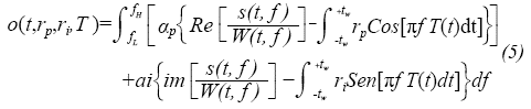
A very narrow window affects resolution in frequency and a very wide window affects resolution in time. If the spectrum of the wavelet W(t,f) is known, r(t) and T(t) may be estimated by optimizing the function fH y hL are the upper and lower limits of the seismic frequency band, and αp and αi are weight functions. The best solution is the one that minimizes equation 5, providing the parameters (rpr¡,T).
Fuzzy Logic Interpolator
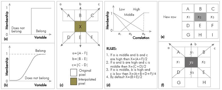
When increasing resolution of an image, the perception of fine details, edges, clarity of objects and image quality increase; an increase that must keep the inherent characteristics of the image. The fuzzy logic theory is used to solve ambiguities and imprécisions caused by linear interpolators in non-linear information in images (edges, fine details, textures, etc.). This branch of artificial intelligence allows handling the complexity of information, based on operating elements of human thought being linguistic tags that may represented in mathematical language through fuzzy sets and associated functions, describing with measurements the behavior of the phenomenon (Ramirez, Barriga, Baturone & Sanchez, 2005). Individuals who belong or do not belong to a classical set and their degree of membership will be 0 or 1 as indicated in Figure la. On the contrary, the probability of belonging to a fuzzy set is estimated by a probability function, as indicated in Figure lb. The function is determined according to the solution given to the problem or phenomenon under study, and therefore is based on expertise.
Figure 1c shows original pixels A, B, C, D, E and F and the X pixel to interpolate, as well as values a, b and с calculated as absolute differences between pixels in each one of the directions (↖,↑,↗). . The function that estimates membership is shown in Figure Id jointly with fuzzy rules that estimate the value of the interpolated pixel X. Three values, α1 α2 and α3, are defined so that correlation is low if it is less than α1, medium if it is between α1 and α2, and high if it is between α2 and α3. Rule 1 assigns to the X pixel the average between pixels A and F if correlation is high in the diagonal (↖), while rule 2 assigns the average between pixels С and D when correlation is higher in the diagonal (↗). Rule 3 estimates an edge in the direction (↑) if correlation is higher vertically and interpolates the average of pixels A, B, C, D; but if correlation is not high, rule 4 assigns the average of pixels В and E. The interpolation process first introduces rows of pixels to be interpolated between rows of original pixels, as in Figure le, where the row of pixels X1x2x3 is inserted between rows ABC and DEF of original pixels. Pixel x2 is interpolated using pixels A, B, C, D, E and F as in Figure 1c, being repeated for the whole row. Then columns are introduced, as in Figure 1f, where column у1у2у3 is inserted between columns Ax1D and Bx2E. The у pixel is interpolated with pixels ABDEGH and the xy pixel is estimated with pixels ABDE and interpolated pixels х1х2у1у3 with the same procedure of Figure 1c. Pixels of the edge of the image are interpolated when averaging the values of their neighboring pixels.
Seismic Attributes
The RMS (Root Mean Square) Amplitude attribute highlights the energy content in a seismic trace and is used to differentiate lithology types, where high RMS amplitude values are related to high-porosity sands (Pereira, Azevedo, Pinheiro & Abbassi, 2009), so it is much used in the oil industry. It is defined as:
Where N is the number of terms in the window, and A is the amplitude of the sample in time (t + k).
The "Sweetness" attribute is used to delimit zones with low-density and high-porosity lithologies, and is defined by the instantaneous frequency (finst) and instantaneous amplitude (Ainst) combination:
Although it is difficult to explain, this attribute represents changes in the form of the seismic trace caused by stratigraphie changes, and has shown good performance in areas where there are impedance contrasts between sand and lutite packages, a reason for which it is very useful to characterize channels (Hart B. 2008).
The variance attribute o, is a measurement of dispersion of a distribution and is defined by:
The variance attribute calculates the difference of value of the trace with the mean value within the window defined by the user and is widely used by interpreters to identify edges or discontinuities (Pereira, L. Azevedo, R. Pinheiro, L., & Abbassi, H., 2009).
3. EXPERIMENTAL DEVELOPMENT AND RESULTS
Values of αp =0.5 and αi , =0.5 were assigned to equate the weight of even and odd components of equation 5. Besides, the Fast Fourier Transform (FFT) was applied in windows of 64 ms centered in 32 ms dimming its edges with Gaussian tapers of 64 ms. A wavelet of 64 ms, representative of the seismic volume, was extracted by auto-correlation of traces. In turn, the genetic algorithm was characterized by the following parameters: size of population, 120 individuals; number of generations, 600; mutation percentage, 0.001; cross percentage, 0.1; allele arrangement of reflection coefficients between -0.35 and 0.35 every 0.01 and allele arrangement of thicknesses (T) between 1 and 30 every 1 ms. The genetic algorithm (AG) of Spectral Inversion was tested with synthetic seismograms where the model, in continuous line in Figure 2a, has layers with thicknesses similar to sandy units with hydrocarbons tested in well.
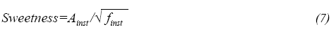
Figure 2 a) Reflectivity series of the model (Red) and estimated reflectivity series (Blue), b) Synthetic trace of the model/ and c) Synthetic trace generated from the estimated reflectivity profile.
The seismogram in Figure 2b results from the convolution of the Ricker wavelet of 80 Hz and the profile of reflectors separated 20 to 30 ms shown in Figure 2a. The continuous lines indicate the coefficients and times of occurrence of the reflectors. On the other hand, the dotted lines are the estimates of Spectral Inversion. Coefficients of the model are very close to the estimates as are the estimated times and those of the model. The foregoing confirms the good performance of the AG to make the inversion of trace of Figure 2b, and differentiate layers as thin as 20 ms. Figure 2c shows the seismogram by convolution of the reflectivity profile estimated with the Ricker wavelet of 80 Hz, which compared to the one of Figure 2b indicates great similarity.
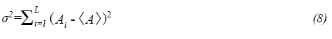
The interpolation algorithm by fuzzy logic was tested in a high-resolution digital image, with pixel of 0.5 m and 256 levels of dynamic range. The image in Figure 3a shows a main channel that splits into branches of different sizes. The image was decimated to obtain another of lower resolution with pixel of lm, to which the interpolation algorithm was applied to restore the original resolution of 0.5, the result of which is shown in Figure 3b. The error by pixel between the image obtained and the original is shown in Figure 3c, regarding which a statistical analysis found that the mean error is 5% with a standard deviation of 3.6%. The error was calculated only in the interpolated pixels, because the original pixels were not modified; and, although the mean error is low, values of 20% were found in the edges of channels and zones with steepest topographic changes.
Figure 3 a) High-resolution digital image with pixel of 0.5 m. b) Image restored with resolution of 0.5m by the interpolation algorithm; and c) Image of error by pixel between the restored image and the original.
The fuzzy interpolation algorithm requires values for α1, α2 and α3, for which the direction of each pixel of the image is calculated as the lowest difference with surrounding pixels. Figure 4a shows the distribution of directions in colors of Figure 3b, while Figure 4b shows the enlargement of the small box with directions of some pixels. The arrow and the color indicate the estimated direction in each pixel and the statistical distribution of directions in the image is summarized in the table of Figure 2c. It shows that the preferential direction is (↖, red) 315° NW-SE with a 54% probability, so the α3 term was set in 0.54%, 24% of pixels have a north-south trend (↑, yellow) so that the α2 term took the value of 0.24 and 0.14 was taken for the α1 term, according to the direction (↗, green). The population of pixels with direction (↔, blue) represents 8% which is the default value.
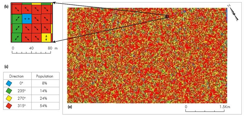
Figure 4 a) Time slice at 864 ms where each pixel indicates a direction in which the difference with respect to its close pixels is minimal, b) Estimated directions in pixels included in the box. c) Distribution statistics of directions in pixels of the map.
Spectral Inversion was applied in the 720 - 920 ms interval of a seismic volume of 20 km2 of the Llanos Basin, focusing on the C7 unit of the Carbonera Formation. The seismic cube was acquired in 2012 by the Pacific E & P company and contains 115 receiver lines pointed at 31° and separated 200 m with group interval of 40 m, 57 source lines pointed at 301° and separated 360 m with sources every 40 m. With a 20 x 20 m2 nominal fold and a maximum offset of 2060 m, the cube covers an area of 366 km2. A Ricker wavelet of 85 Hz was used and the search space was restricted as well as the reflectivity profiles which represent the individuals of the initial population. Figure 5 a shows a seismic section of the XLINE 600 in strike direction, located between INLINES 610 and 685, and in the 800 - 950 ms interval. Figure 5b contains the image of line 600 after the inversion. An increase in vertical resolution is observed, which is shown with more lateral continuity of reflectors, particularly strong reflectors at the top of C7 at 835 ms as well as the Pre-Cretaceous unconformity at 880 ms. Figure 5c shows the amplitude map of the time slice at 864 ms close to the top of the C7 unit, while Figure 5 d contains the amplitude map of the time slice at 864 ms after the Spectral Inversion. It is observed that there is a better delimitation of what could be interpreted as a channel in the circle of yellow color of Figure 5c and 5d. Figure 6 shows sandy and lutitic units interpreted by the Gamma ray record of well A, the tops of which look adjusted to well defined reflectors in the seismic image subsequent to the inversion. Reflectors define sandy packages between the top of C7 unit and the Pre-Cretaceous unconformity in the 864 ms - 910 ms interval and those of C6 unit between 842 and 860 ms, as well as the thin lutitic units in C4 and C5 units. Sand packages in yellow color have thicknesses between 10 and 30 feet which are lower than the 24 feet of seismic resolution of the original cube. The interpolation algorithm with fuzzy logic was applied to the seismic volume provided by seismic Spectral Inversion.
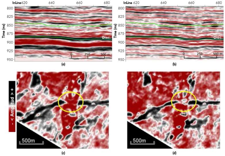
Figure 5 a) Seismic section of the XLINE 600 in direction perpendicular to the dip that shows the top of the C7 unit of the Carbonera Formation and the Cretaceous unconformity, b) Seismic section in direction perpendicular to the dip after applying the inversion, c) Amplitude map of time slice at 864 ms before the inversion; and d) Amplitude map of time slice at 864 ms after applying the inversion.
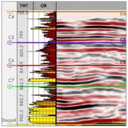
Figure 6 Gamma Ray record of well A with sandy and clayey packages interpreted in the column/ which are tied to well-defined reflectors in the seismic image subsequent to the inversion.
Figure 7a shows the map of amplitudes at 864 ms before the inversion and Figure 7b shows the map at 864 ms after applying inversion and interpolation. As a result, more continuity and smoothing of edges is achieved, particularly a structure that crosses the image to the right, from the bottom up. This effect is better observed when comparing images 7c and 7d which are enlargements of the boxes in Figures 7a and 7b, where interpolation smoothes the edges and better defines the geomorphological structures allowing a better delimitation and stratigraphie interpretation.
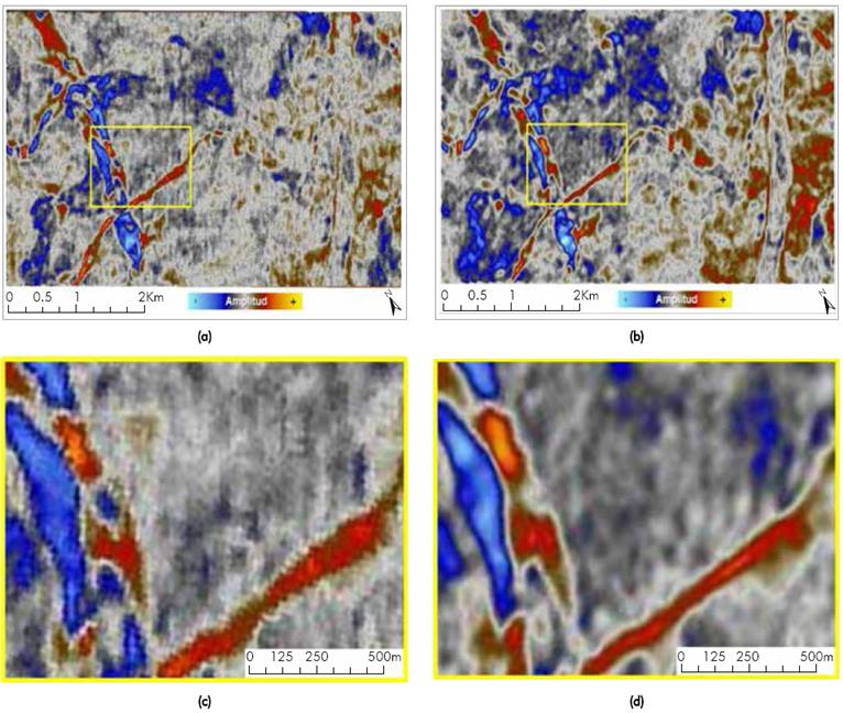
Figure 7 а) Amplitude тар of time slice at 864 ms without applying inversion or interpolation/ b) Map of amplitudes of time slice at 864 ms after inversion and interpolation with fuzzy logic/ c) Enlargement of box in Figure 5a, and d) Enlargement of box in Figure 5b.
Seismic Attributes
A calculation was made of volumes of RMS-Amplitude and Sweetness attributes by their sensitivity and response to stratigraphie features, and the volume Variance attribute by the capacity to highlight structural discontinuities like channel edges, faults and fractures. Attributes were calculated with short and long time windows to select their optimal parameters, and from the analysis thereof a window of 10 ms was chosen for the RMS-Amplitude attribute, a window of 12 ms was chosen for the sweetness attribute, and a size of 12 samples in a time window of 6 ms was chosen for the attribute of Variance.
A study was made of the effect of the seismic attribute of variance on highlighting of geomorphological structures and the effect of the sweetness attribute to discern sands from lutites in the flattened cube at the top of the C3 unit as reference surface. In a first step, variance was estimated in the seismic volume and in the volume after inversion plus interpolation. Figure 8a shows the variance map at 864 ms without inversion or extrapolation while Figure 8b displays the variance map at 864 ms after inversion and extrapolation. Figure 8b shows with more sharpness the edges of geomorphological structures present in such time, highlighting what is evidenced as a system of meandering distributary channels in direction East-West and other rectilinear channel in direction North-South. In a second step, an estimate was made of sweetness in the seismic volume and in the volume resulting from inversion and interpolation; and to assess its impact the sweetness map was overlapped on the variance map. Figure 9a shows the map at 864 ms of sweetness with variance without inversion or interpolation, while Figure 9b contains the map at 864 ms of sweetness with variance, and with inversion and interpolation. A better performance of this attribute is seen in data after applying inversion and interpolation, differentiating sands (associated with positive values) from lutites (associated with negative values), which makes interpretation easier.
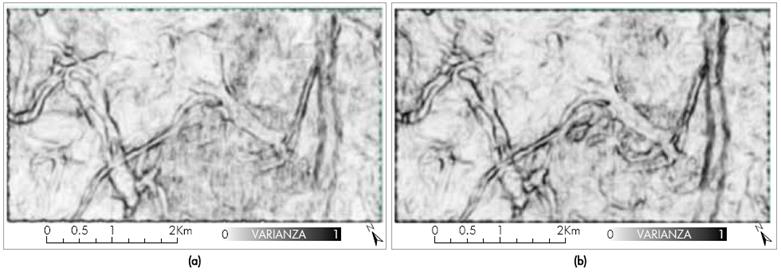
Figure 8 a) Variance of the map at 864 ms without applying inversion or interpolation, b) Variance of the map at 864 ms after applying Spectral Inversion and interpolation.
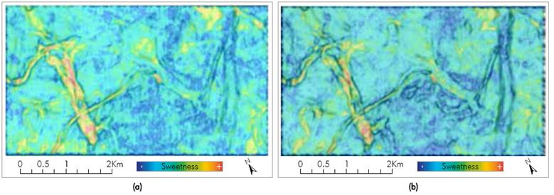
Figure 9 a) Image of sweetness overlapped with variance of the map at 864 ms without applying inversion or interpolation, b) Image of overlapping of sweetness with variance of the map at 864 ms with Spectral Inversion and interpolation.
Overlapping of both attributes was used in the geomorphological interpretation of the maps to identify channels and other stratigraphie features (Hart, 2008); using a window of 12 ms (6 ms above and 6 ms below each map). Maps at 902, at 886 and at 864 ms were geomorphologically interpreted, being shown in Figures 10a, 10b and 10c, respectively. In the map at 902 ms (Figure 10a), two distribuitary channels, one main channel with overflowing zones and accretion zones, and a flooding zone are identified. Figure 10b shows the map at 886 ms, where there is an interpretation of a flood plain and an erosion zone with the presence of sands, differentiated by sweetness with yellow to red colors. In the map at 864 ms, contained in Figure 10c, two river systems are interpreted: in blue color, a system of braided channels in north-south direction, and the other in violet color, characterized by thin channels related to events of lower energy in east-west direction; and associated with this system an overflowing zone was interpreted, delimited by the presence of sands identified by sweetness. The foregoing interpretations are consistent with the environments reported in wells A and B, which are shown in the three maps. Figure 10d shows a seismic dip section indicating the three maps crossed by well A. The interpretations of channel systems described above are contextualized in the regional geological framework of the Llanos Basin for the Carbonera formation, which is characterized by the presence of river environments of high and low energy, so that the applied methodology provides information that contributes to the interpretation of fine strata of geological features, such as channels, overflowing zones, flood plains and abandoned channels.

4. CONCLUSIONS
To increase temporal and spatial resolution of 3D seismic, Spectral Inversion and interpolation with fuzzy logic algorithms were implemented, which tested in synthetic seismograms and in a high-resolution image showed great performance. Spectral Inversion resolves strata with thicknesses lower than those observed in the original seismic section, which could be verified when comparing the seismic image subsequent to inversion to interpreted well records. When assessing the performance of the interpolation algorithm with fuzzy logic in the high-resolution image it was found that a value equal to the one expected may be interpolated with a probability of success of 95% with a standard deviation of 3.6%, which indicates high confidence in its prediction.
However, the error is increased due to lack of continuity in the edges and in the case of sudden changes. Joint application to a seismic volume of the Llanos Basin increased volume resolution, which allowed geological interpretation of three maps at different times, which was confirmed with well records. Tests in volumes before and after the process indicate that the seismic attributes used allow a better display in seismic maps with higher resolution. Although the application of this interpolation method is unknown in the improvement of lateral resolution in seismic maps, its use in this project shows its usefulness for this purpose.

