


 English (pdf)
 Article in xml format
 Article references
 Send this article by e-mail
 Cited by SciELO
  Cited by Google
  Similars in
SciELO
Similars in
SciELO  Similars in Google
 Permalink
1. INTRODUCTION
Bubble bed bioreactors are important for the food industry, bioprocesses, pharmaceutics, oil chemistry, bio fuels purification, wastewater and effluents treatment[1]-[3]. Recently, these devices have gained great interest due to their versatility and application potential. In a bioreactor, a gas phase is bubbled though a liquid bed to induce mass transfer. A bioreactor efficiency depends on the available surface area [4], [5]. Therefore, to enhance mass transfer it is necessary to reduce bubble diameter in an efficient manner[6]-[8]. One possible method to reduce bubble size is to use micro diverter valves to feed the gas to the system(1). Micro-diverter valves limit bubble growth using an oscillatory gas flow supply [9].
Micro-diverter valves have been tested at Reynolds numbers between 800 to 15000, producing oscillatory microbubble flows with frequencies ranging from 1 to 200 Hz. Several geometrical variables can be tuned to enhance the performance of the fluidic oscillation process [6]. In a recent publication, the methods for micro and nanobubble generation were evaluated[10]. The geometrical parameters of the valve have been set to feed microalgae with a CO2 concentrated exhaust gas in the form of dispersed microbubbles [11]-[12]. However, these valves have not been tested for other applications, due to the intricacies of the design. Indeed, depending on the application, the geometry of the device is modified to impose different bubbling regimes. Due to the complexity of the flow in these devices, a simulation stage is needed prior to fabrication. Thus, a reproducible modeling approach based on the detailed fluid transport phenomena is required. This is the main objective of the present study.
Fluid behavior inside micro diverter valve has been studied at the micro scale by means of CFD simulations due to the complexities involved: turbulence, compressibility, oscillation, unsteady state and size scale. Suitable and efficient CFD modeling makes possible to evaluate multiple conditions, reducing experimental work and development costs [13]. For example, the flow diverting process at low Reynolds numbers has been studied through CFD techniques [12]. Experimentally, the fluidic oscillator has been assessed in a wind tunnel to understand the pressure recovery in the equipment, which directly affects the energy efficiency [14]. This feature reduced costs in the process, as compression costs are important in bioprocesses. CFD simulations have been compared against experimental results obtained from Particle Image Velocimetry (PIV) tests [15], demonstrating the possibility of using CFD modeling to increase the performance of the device . Mesh adaptation methods have been used to reduce the error associated with the mesh resolution and processing computation limit [15].
Despite the efforts made in recent years to evaluate valve performance by means of CFD simulations, detailed CFD numerical modeling and evaluation has not been performed due to the high computational requirements and complexity of turbulence behavior modeling in oscillating systems. An evaluation of mesh generation methods and a mesh independence analysis has not been carried out because this procedure involves a lengthy preprocessing time. Moreover, turbulence models, which may affect results and influence computation time, have not been assessed in detail. These reasons make this study an important one regarding the CFD modeling of the system, establishing a foundation for further development worldwide in several industrial applications.
This paper presents the CFD modeling evaluation of a bi-stable diverted valve at a Reynolds number of 3800 and a frequency of 200 Hz. First, two mesh generation methods were evaluated to simulate this valve at steady state condition. Then, a mesh independence analysis was carried out to find an adequate mesh size and a configuration with a reasonable computational time and accurate results. A brief analysis regarding time-step size using the Courant number approach was also performed. Subsequently, the transient behavior of the valve was reproduced and analyzed by simulating successive steady states, using the pseudo-steady state approach. Finally, results obtained using two turbulence models (k - ε Standard and RGN) were compared [16]-[17]. The behavior of the flow process in the system is presented. The results will be compared and validated using experimental data in a future publication.
2. EXPERIMENTAL DEVELOPMENT
MICRO-DIVERTER VALVE MODEL
The micro diverter valves presented have geometric characteristics that contribute to flow deflection[12]. First, the fluid enters the equipment through the supply terminal S (Figure 1). Second, the valve has a contraction that transforms pressure energy into kinetic energy; a lower pressure causes further flow deflection. Next, a recycled stream impinges upon the flow coming from the contraction, and causes its deflection.
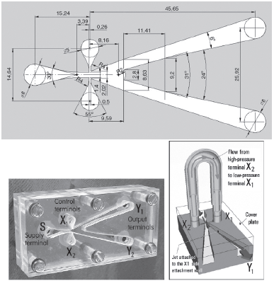
Subsequently, in a pressure recovery expansion region, the flow attaches to one wall, and enough turbulence is generated to decrease the pressure in the opposite wall. This causes the main flow to exit the valve trough the terminal close to the high-pressure region. At the same time, flow enters the valve through the terminal close to the low-pressure region, where the curved splitter nose diverts fluid layers back towards the outlet of the contraction. This holds the flow deflected before it moves to the opposite wall [15].
OPERATION AND BOUNDARY CONDITIONS
Industrial processes require the highest possible mass transfer, and this is achieved by reducing the bubble size. Microbubble diameter depends directly on the fluidic oscillation frequency. The valve operation frequency ranges from 1 to 200 Hz. The higher the frequency the lower bubble size [12]. Therefore, in this work a frequency of 200 Hz is used. At higher frequency, there are faster pressure changes in the equipment and it is more difficult to reproduce the fluid behavior in the valve. Experimental work shows pressure recovery occurs properly at Reynolds numbers higher than 10000 [14]. However the valve works properly at Reynolds numbers above 2000 [15]. In this work, a Reynolds number of 3800 was used.
This article evaluates the valve at best operating condition to divert 20 L per min of air (200 Hz). The velocity at the supply terminal S is 12 m/s (Figure 1). The pressure at outlets Y1 and Y2 is fixed at 0 Pa. In order to find stable states, the recycle was not considered and control terminals XI and X2 were replaced by walls. Later, the recycle was taken into account to simulate transient states,
MATHEMATICAL MODELS
Ansys-Fluent® was used to model the system (version 14.0). In Ansys-Fluent the finite volume method is used to solve continuity and momentum equations in tridimensional Cartesian coordinates over an unstructured tetrahedral mesh. The turbulent behavior was calculated using the two equation k-epsilon model in the standard and RNG formulations, and the latter model is suitable for handling "soft" swirling flows and low-Reynolds number effects [17]-[22] Standard wall functions treatment was used to solve turbulence stresses, and the turbulence model constants were not modified.
Second order upwind for momentum, and first order upwind for turbulent kinetic energy and dissipation rate were implemented as discretization schemes. The SIMPLE algorithm was used for pressure-velocity coupling. The equations were solved using default under-relaxation factors, and they were adequate to solve continuity equations with residuals of which are consistent with values reported elsewhere for similar simulations [15]. The simulations were carried out using high power hardware, and the main specifications of the workstation equipment used are as follows:
MESH INDEPENDENCE ANALYSIS
In previous works, stationary states for the valve have been modeled to study the scalability properties of the equipment, in terms of dimensionless numbers, to analyze the pressure recovery Inside the valve and to calculate the pressure difference that generates fluidic oscillation [12], [14]-[15], Other studies have performed evaluations of accuracy for modeling In steady state fluid flows avoiding turbulent considerations, and this approach has made it possible to estimate the error associated with mesh performance [23]-[25], In these works, steady states for the equipment were used to analyze pressure and velocity profiles using gradient adaptation refinement. If boundary conditions are not changed, this refinement method is suitable for calculating profiles in regions with abrupt changes. For problems with changing boundary conditions and flow oscillation, a gradient adaptation procedure would increase computational time due to the continuous change of gradient positions. Instead, the system can be modeled using a constant mesh over which different boundary conditions are imposed. This approach was used in this study.
Tetrahedral meshes were created using advanced size function. To increase control over cells sizes, the angle between normal vectors, the number of elements used in the gaps, and the progression between minimum and maximum cell size were changed[17]. The curvature, and proximity and curvature methods were employed Patch conforming tetrahedrons were used for local control of the mesh.
These procedures were Implemented to generate meshes with gradually Increasing cell numbers ranging from 10 xlO3 to 1500 xlO3 elements. In order to evaluate mesh Independence, errors were computed using equations (1) and (2).
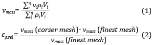
Where v mass is the mass weighted average velocity, and εp,rel is the mass weighted velocity relative error of the domain, v¡ is the velocity (L/T3), p¡ is the density (M/L3), and V, the volume of the cell I (L3). A total of 18 meshes of different sizes were tested for the curvature method, and 14 for the proximity and curvature method. Table 1 sets out a review of previous studies where different refinement methods were used to simulate this valve. As can be seen, meshes from 17xl03 to 200 xlO3 cells were evaluated. In this work, a wider number of cells were examined.
Table 1 Cells number and refinement methods used in different studies.
| Author | Number of Cells | Refinement method |
| Tesar, V., C.-H. Hung, et al. (2006) | 70 x 103 | Not Reported |
| Tesar, V. (2009) | 17 x 103- 30 x 103 | Gradient Adaptation |
| Tesar, V. and H. C. H. Bandalusena (2011) | 150 x 103 - 200 x 103 | Gradient Adaptation |
| This study | 10 x 103-1500 x 103 | Advanced size function and gradient adaptation methods |
3. RESULTS AND ANALYSIS
MESH INDEPENDENCE ANALYSIS
Figure 2 shows that even at a low number of cells, the mass weighted velocity relative error is acceptable (less than 18%). Both cell size function methods, curvature and curvature and proximity, show that the error decreases when the number of cells increase. However, curvature and proximity shows a monotonic decreasing trend and thus this method was chosen for further evaluations.
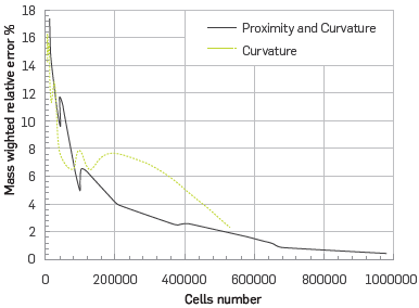
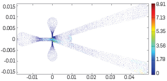
Figure 2 only shows the global error for the valve. Nonetheless in regions with abrupt gradients, errors may be higher and thus it is necessary to study these regions in greater detail. The results of these analyses are presented in Figure 3, which sets out the difference between velocity vectors obtained using a mesh of 681000 cells and coarser meshes in all regions of the valve. In order to compare velocity profiles obtained from different meshes, the velocity was interpolated [19]. The velocity differences at output terminal Y1 are small, and this is because the flow was low at that terminal. As expected, velocity differences are higher in regions with abrupt gradients as at the pressure recovery expansion region, and especially near the walls.

Figure 3.Velocity vectors difference (m/s) between the velocity profiles obtained using meshes of 12000 (Up-left), 41000 (Up-right), 106000 (Down-left), 368000 (Down-right), and a mesh of 681000 elements.
A velocity relative error, calculated using equation (3), was used to compare the results obtained from different meshes.
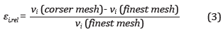
Where ε ¡,rel is the velocity relative error at cell i. In specific regions, velocity relative errors decrease from 30 to 10% as the cells number increases. These errors are not significant and only occur in specific zones of the valve. Thus coarser meshes could be used to simulate this valve. Nevertheless, this study was accomplished using a regular commercial computer, and even if higher precision is required, this can be accomplished with the same computational power. A mesh with 681067 elements had a mass weighted velocity relative error lower than 1 % and was used in further simulations.
TIME-STEP ANALYSIS
A time-step analysis based on the Courant number approach was performed to establish the suitable time-step range for CFD simulations for this kind of flow device. The courant number is defined as:
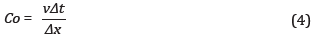
where v is the greatest velocity magnitude (50 m/s), in this case the maximum velocity expected inside the device at high Reynolds number values, Δt is the time-step in S, and Δx is the mean cell size (4.58 x 10⁻⁴ m). The recommended Co number values for the simulation to converge is: 5<Co<30. This is according to the cases developed for similar flows reported in literature[17]-[19].
For this condition and the conditions mentioned above, it is possible to estimate the range of time-step for the simulations performed: 4.58x10⁻⁵s< Δt<2.75 x10⁻⁴ s. This range can be used as reference for the set-up of the simulations. Additional parameters, such as mesh size and computational power available must be considered. The analysis presented in this section could be used to reproduce the transient simulations of oscillatory turbulent high Re micro-scale flows, adding information that can be supplemented by other studies focused mainly on the numerical error due to mesh performance[23]-[25].
COMPARISON BETWEEN ADVANCE SIZE FUNCTION AND GRADIENT ADAPTATION MESH GENERATION METHODS
For problems with changing boundary conditions and flow oscillation, a gradient adaptation meshing method would increase computational time due to the continuous change of gradient positions. Since, in this study, states with different boundary conditions were simulated, advance size functions were used to simplify mesh generation. In this section, both mesh generation methods are compared. Figure 4 shows interpolated vectors colored by velocity difference between the velocity profiles obtained using advance size function (681067 cells) and gradient adaptation methods (609000 cells). This figure shows that differences between both methods are small; the higher velocity relative errors are smaller than 8% and occur after the contraction nozzle. Therefore, usage of the advance function method is adequate to simulate the valve at different states and thus it was used in further simulations. It is important to mention that both methods have very similar average orthogonal qualities (0.84 and 0.86).
OSCILLATING FLOW DESCRIPTION
First, an attempt was made to simulate the flow at transient state using temporal discretization, the unsteady solutions methods, and the k - ε turbulence model. However, the flow oscillation was not observed even using the finest meshes. It seems that the k - e turbulence model does not reproduce fine details of the turbulence generated in the valve. An advanced turbulence model could be used in future studies to describe the details of the turbulent phenomena.
In order to simulate the transient behavior of the equipment, a set of consecutive steady states were simulated[15]. The boundary conditions at terminal X1 and X2 were imposed using reported experimental data. To do this, the flow at one control terminal was increased for different steady states until the main flow diverted towards the opposite wall. Then, the recycle flow was decreased in that control terminal until zero. The same procedure was repeated in the opposite control terminal. A succession of these recycle flow pulses holds the flow oscillating continuously.
In a steady state simulation, depending on boundary and initial conditions, the main flow may attach to one wall or the other. Figure 5 shows pressure distribution at the pressure recovery expansion zone for four states. As the velocity increases at the wall where the main flow is attached, the pressure decreases [Figure 5, upper-left). Then, the pressure gradient between the control terminals drives a flow toward the terminal where the main flow is attached (Figure 5, upper-right). This flow destabilizes and detaches the main flow. Later, the main flow diverts towards the opposite wall (Figure 5, lower-left). Subsequently, as the main flow attaches to the opposite wall, the pressure profile inside the recycle inverts and the flow inside the recycle changes its direction from one control terminal to the other (Figure 5, lower-right).
Both valve outlets have nearly the same pressure. High turbulence at the pressure recovery expansion reduces pressure and causes oscillating flow entry at terminals Y1 or Y2. Main flow velocity at the inlet is 12 m/s and at terminals Y1 or Y2 it is near to 17 m/s. This increase is caused by pressure reduction in the equipment and the additional flow entering terminal Y1 or Y2.
The recycle acts as a feedback control loop that destabilizes, detaches and moves the main flow from one wall to the opposite wall. It acts as a signal transmitter that connects control terminals X1 and X2. Flow at the recycle is the control element, which is used to destabilize the main flow by imparting momentum on it. The velocity after contraction is higher and pressure is lower, thus a small change in pressure after the contraction can easily modify the main flow. The recycle control is enhanced by the geometry of the pressure recovery expansion as the detachment process is retarded by the action of streams deflected by the curved splitter nose [15].
Previous studies used Reynolds numbers from 800 - 15000. These studies proved that even at a low Reynolds number, the vortex in the pressure recovery expansion oscillates and the diverting process occurs. In this study, we used a Reynolds number of 3400, and the diverting process was observed as expected. At this Reynolds, a pressure loss of 1000 Pa was observed, and such pressure loss did not affect the diverting process. This pressure loss does not seem to be significant, however, if several valves are to be used in parallel or a series, consideration must be given to ensuring good hydraulic behavior in the system.
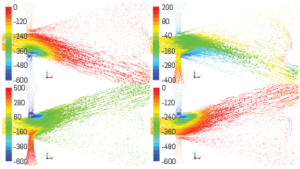
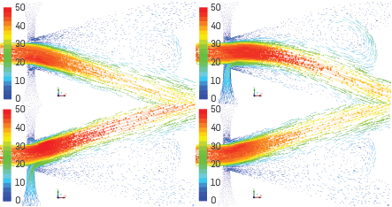
Figure 6 shows the velocity distribution at the pressure recovery expansion zone. The first state was simulated using walls as boundary conditions at the recycle terminals, thus fluid velocity in the terminals was zero (Up-left). Later, the velocity was increased gradually at the terminal next to the wall where the main flow was attached. The velocity of the recycled fluid was increased from 0 to 2.5 m/s, in steps of 0.12 m/s, until main flow was diverted to the other output terminal (down-left). After this happened, the velocity of the recycled fluid was decreased, using the same step, until zero (down-right). This process takes around 2.5 ms. At the end of the process, the velocity of the recycled fluid starts to increase at the opposite terminal until an oscillation is completed. A supplementary video shows the process (Video 1 k epsilon RNG: https://www.youtube.com/watch?v=GyW97mvbreo).
COMPARISON OF k - ε STANDARD AND k - ε RNG TURBULENCE MODELS
The K - ε standard model is a simple approach that can predict turbulent energy and its dissipation rate locally along the flow domain. However, this model is not suitable for rotating flows with large strains [8]. The k - ε RNG formulation is effective to simulate small-scale turbulence inside expanding ducts with higher accuracies. Since k - ε RNG is able to reproduce turbulence in more complex processes, it has been used to simulate intricate flow patterns inside expansion ducts. However, the computational cost of this model is higher than the k - ε standard model. In this section, we aim to compare these two turbulence models.
Figure 7 shows the ratio of outlet flow to supply flow as a function of time. This figure shows that there is a 20% overflow at outlet terminals, and the opposite outlet provides this overflow. The entering flow moves to the low-pressure region of the pressure recovery expansion and helps to increase the momentum of the recycle flow. This is consistent with experimental overflows of 17% reported in other studies [15]. A comparison of k- ε standard and K - ε RNG results shows that both turbulence models predict the same mean behavior (Figure 7), however, k - ε RNG reproduces the oscillating fluctuations over the mean. The main difference between both turbulence models is the computation time, as calculations with k - ε standard required half the time required with the K - ε RNG model. Therefore, the k- ε standard model is able to reproduce turbulence in the device at a Lower computational cost.
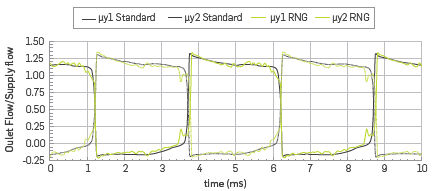
Figure 7 Ratio of outlet flow to supply flow as a function of time. Comparison of K - s standard and k - s RNG turbulence models (py= Outlet flow/Supply flow).
Figure 8 shows the ratio of the recycled flow at terminals XI and X2 to supply flow. Since information about the flow at terminals XI and X2 was not available, this flow was linearly increased and decreased with time. The flow was increased until the main flow diverted. The simulations showed that the recycled flow must be 14 % of inlet flow to deflect the main flow; this result is higher than the 7 % reported in other studies [20]. This difference is due to the higher viscous effects occurring at the lower Reynolds number used in this article[17]-[19].
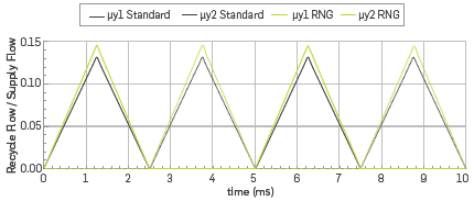
Figure 8 Ratio of recycled flow to supply flow as a function of time. Comparison of K - ε standard and k - ε RNG turbulence models (px=Recycle flow/Supply flow).
The results show a good qualitative representation of the oscillatory and highly unstable flow pattern. Velocity profiles of the transient simulations for both turbulence models can be seen in: Video 1 k epsilon RNG:
https://www.youtube.com/watch?v=GyW97mvbreo
Video 2 k epsilon standard:
https://www.youtube.com/watch?v=NhQ_jFvPwMY
This description of the system makes it possible to understand the microscale effect of the flow oscillations. This model can be used to tailor the properties of the micro diverter valve to sustain the fluid oscillation required in different bubbling regimes. A validation of this model will be presented in a future study.
WALL FUNCTION Y + ANALYSIS
The effect of the wall function y+, known as dimensionless wall distance, is discussed in this section. In the modern CFD modeling approaches of turbulent flow, the y+ variable is not explicitly used. y+ is a variable that can be calculated from CFD results. In other words, in the actual CFD modeling approach, y+, which makes it possible to model the boundary layer behavior in detail, is not used because it is a classic technique that limits the possibilities of mesh inflation and the capability of the CFD model to accurately reproduce pressure and velocity.
Furthermore, due to the non-stable nature of oscillating flow patterns in this study system it is not possible to use wall functions. This because the variability in the velocity fields cause the boundary layer size to change frequently in a way that cannot be described correctly by the wall function y+, and doing so would cause an error in the flow field, as can be seen in Figure 9b.
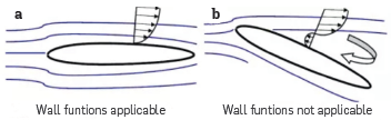
Figure 9 Applicability of wall functions: (a) Wall functions applicable case phenomena, and (b) Wall functions not applicable case phenomena. Taken from [26].
The implementation of any wall function will require further development in the boundary layer theory, making this classical approach suitable for this highly unstable oscillating flow modeling. Meanwhile the CFD modeling approach with high quality mesh performance is the best way to evaluate (in detail) the flow behavior to capture the boundary layer effects in detail.
CONCLUSIONS
The CFD modeling evaluation of a no-moving parts bi-stable diverted valve was presented. First, transient and steady state approaches were used to reproduce the fluid behavior in the valve. Different mesh configurations, mesh generation methods, and two turbulence models were evaluated to find the most adequate setup to simulate this valve within reasonable computational times and acceptable errors. Finally, operation conditions at a low Reynolds (3800) and a high frequency (200 Hz) were used to assess other possible applications.
The evaluation of the mesh generation methods showed that both methods produce nearly the same results at steady state conditions. However, in transient state the gradient adaptation method would increase computational time due to the continuous mesh refinement caused by the change of gradient positions. Meshes from 10000 to 1600000 cells were used to evaluate the mesh independence. The errors observed between coarser and finer meshes are not significant and only occur in specific zones of the valve, thus coarser meshes could be used to simulate this valve. An estimated time-step range for the simulations performed was obtained: 4.58x10⁻⁵s< Δt<2.75 x10⁻⁴s. This range can be used as reference to set-up the simulations. Additional parameters, such as mesh size and computational power available must be considered.
Transient flow in the micro diverter valve was simulated using temporal discretization, unsteady solution methods, and the k - ε turbulence model. However, the flow oscillation was not observed in detail, even when using the finest meshes. The transient behavior of the equipment was evaluated using a set of consecutive steady states, with the recycled flow imposed as a boundary condition. The use of this approach showed that it is possible to reproduce the flow oscillation through consecutive steady states.
A comparison of k-ε standard and k - ε RNG results shows that both turbulence models predict the same mean behavior. However, the k - ε RNG reproduces the oscillating fluctuations around the mean. Nonetheless, calculations with k- ε standard took half the time than the computation using the k - ε RNG model. Therefore, the k- ε standard model is more adequate to simulate this valve with limited computational resources.
The results for this work also show that even at a low Reynolds number (3800) and a high frequency (200 Hz), the valve was able to divert the fluid. Thus, this valve is a robust and flexible device that can be used in a wide number of industrial applications. CFD proved to be a powerful tool to evaluate different configurations reducing experimental work. The results show the qualitative behavior of the fluid phenomena involved in the system.
Further research is required to apply wall functions such as y+ in a suitable manner for this case, without making conceptual mistakes in relation to inaccurate modeling, mainly in the boundary layer.

