English (pdf)
 Article in xml format
 Article references
 Send this article by e-mail
 Cited by SciELO
  Cited by Google
  Similars in
SciELO
Similars in
SciELO  Similars in Google
 Permalink
1. INTRODUCTION
In this paper, we provide a new and comprehensive perspective on primaries and multiples, that encompasses both removing multiples and using multiples. We describe the original motivation and objectives behind these two initiatives, viewed almost always as "remove multiples versus use multiples". The premise behind that "versus" phrasing speaks to a competing and adversarial relationship. A contribution in this paper is placing these two activities and interests within a single comprehensive framework and platform. That in turn reveals and demonstrates their complementary rather than adversarial nature and relationship.
They are in fact after the same single exact goal, that is, to image primaries: both recorded primaries and unrecorded primaries. There are circumstances where a recorded multiple can be used to find an approximate image of an unrecorded subevent primary of the recorded multiple.
All direct methods for imaging and inversion require only primaries as input. To image recorded primaries requires that recorded multiples must first be removed. To try to use a recorded multiple to find an approximate image of an unrecorded primary subevent of the recorded multiple requires that unrecorded multiple subevents of the recorded multiple be removed. All multiples, recorded multiples and unrecorded multiples need to be removed. Not removing those recorded and unrecorded multiples will produce imaging artifacts and false and misleading images, when seeking to image recorded and unrecorded primaries, respectively.
For indirect methods that either: [1] solve a forward problem in an inverse sense, like AVO or [2] are model matching methods like, e.g., FWI, any data can be forward modeled and solved in an inverse sense, or model matched, respectively. In contrast, for direct inverse methods the data required and the algorithms called upon are explicitly and unambiguously defined.
In our view, direct and indirect methods each have a role to play, the former where the assumed physics (and an assumed partial differential equation governs the wave phenomena) captures some component of reality and the latter (indirect methods) is the only possible choice for the part of reality that is beyond our physical models, equations and assumptions. Furthermore, it would be ideal if the indirect method and the direct method were cooperative and consistent. That cooperation can be arranged by choosing the objective function or sought after quantity to be satisfied (in the indirect solution) as a property of the direct solution [1].
In this paper, we depend upon the clarity of direct methods to provide a new perspective that advances our understanding of the role of primaries and multiples in seismic exploration. That, in turn, allows us to recognize the priority of developing more effective multiple removal capability within a comprehensive strategy of providing increased seismic processing and interpretation effectiveness. The unmatched clarity and definitiveness of direct inverse methods provides a new, unambiguous and clearer perspective with a timely message on the role of primaries and multiples in seismic processing for structural determination and amplitude analysis.
STATE OF THE TECHNIQUE
DIRECT AND INDIRECT METHODS FOR STRUCTURAL DETERMINATION AND AMPLITUDE ANALYSIS
The starting point of our discussion of primaries and multiples begins with the key definitions and classification of direct and indirect inversion methods.
Inverse methods are either direct or indirect (see, e.g., the definition and examples of direct and indirect inversion in e.g., [2], [3]. Direct methods provide assurance and confidence, that we are solving the problem of interest. For example the direct solution of the quadratic equation ax 2+bx+c=0 has roots x=(-b±√(b2-4ac)/2a). Nobody would consider an indirect solution of the quadratic equation. The clear logic and reasoning behind choosing a direct solution of the quadratic equation [where indirect solutions of guessing roots, and matching and minimizing cost functions, e.g., to seek values of x to minimize (ax 2+bx+c)n n or integrals of such an expression] carries over to all math and math-physics problems (including inverse seismic problems) wherever a direct solution exists.
HOW TO DETERMINE WHETHER A PROBLEM OF INTEREST IS THE PROBLEM WE (THE PETROLEUM INDUSTRY) NEED TO BE INTERESTED IN?
In addition to knowing that we are solving the problem of interest, and equally important, direct solutions communicate whether the problem of interest is the problem that we (the petroleum industry) need to be interested in. When a direct solution does not result in an improved drill success rate, we know that the problem we have chosen to solve is not the right problem since the solution is direct and cannot be the issue. On the other hand with an indirect method, if the result is not an improved drill success rate, then the issue can be either the chosen problem, or the particular choice within the plethora of indirect solution methods, or both.
Among key aspects in effectively designing and managing an industrial or academic research program, are: (1) to be able to identify and select the problems and challenges that need to be addressed and (2) what benefit would derive from a new and effective method that addresses a specific challenge. From our perspective, benefit is measured by an increase in successful exploration drilling and optimizing appraisal and development drill placement. Challenges arise when the assumptions behind current seismic methods are not satisfied. As noted in the previous section, direct methods play a unique role in problem identification, a critical aspect of defining research objectives and programs.
THE DISCONNECT BETWEEN THE SUCCESS RATE OFTEN CLAIMED BY RESEARCHERS AND THE REALITY OF THE DRILL SUCCESS RATE IN DEEP WATER FRONTIER EXPLORATION
In our experience, the most important ingredient in defining challenges, and prioritized open issues that need to be addressed is asking the end-user [e.g., the seismic interpreter, the drill decision makers in operating business units] what methods are [and are not] working, and under what circumstances. These individuals by and large only have the single interest and objective in their focus on effectiveness, avoiding dry-holes and making successful drill decisions. On the other hand, there is too often a serious disconnect between, e.g., the frontier drill success rate of 1 in 10 in the deep water Gulf of Mexico and the 100% success rate typically reported by researchers at international professional conferences and in societal publications. Too often, researchers will simply refuse to recognize major problems and challenges that exist, unless and until they might feel comfortable they can address them. That avoidance of recognizing major challenges and obstacles is what we call "the disconnect". Within that "disconnect" resides a tremendous positive set of opportunities to define major E and P challenges and to address them. Seeking funding can be tricky, since we are directed to research departments for that support. There will often be one individual (or at most a very small number) within a research organization who is (are) able to recognize prioritized and significant pressing challenges and problems and is fascinated rather than frightened by new visions of what might be possible. We have been enormously fortunate for the funding and support we have received and do receive, and we are enormously grateful and deeply appreciative.
RELEVANT RESEARCH PROGRAMS BEGIN BY DEFINING CURRENT SHORTCOMINGS AND ADDRESSING ACTUAL SEISMIC CHALLENGES
In our view a research program needs to begin by defining the actual real world seismic challenges and pressing issues, and the current method shortcomings being addressed | and then developing and delivering methods that address those challenges. A relevant research program must begin with the problem, and then seeks a solution; it does not involve a method looking for a problem.
We encourage and welcome and need new seismic methods and capability. However, in our view, all new ideas for imaging and inversion (e.g., interferometry and Marchenko and virtual sources), need to begin by clearly defining the shortcoming and limitation of current capability that they are addressing. And they need to specifically define the challenge and potential added value relative to the current high water mark of imaging and inversion methods that is, Stolt Claerbout III migration-inversion, for automatically and simultaneously imaging and inverting specular and non-specular reflectors (curved reflectors, diffractors and pinch-outs) see, e.g., [4], [5] and the inverse scattering series (ISS) task specific subseries for depth imaging and inversion, [6], where the former (Stolt CIII) require and the latter (ISS methods) do not require subsurface information, respectively.
There is too often an insular inward looking aspect to research projects that do not deem it necessary to show relevant differential added value relative to current capability. In our view, that is essential | and it is incumbent upon us as researchers to explain where a new advance sits within the seismic toolbox, and the circumstances when it will be (and will not be) the appropriate and indicated choice among method options. The research objective is to increase tool-box options.
All of our research reporting needs to have the method assumptions clearly spelled out in the conclusions, and to delineate the remaining open issues that need to be addressed and will require new concepts and future contributions.
MULTI-D DIRECT INVERSION
The inverse scattering series (ISS) is the only direct inversion method for a multidimensional subsurface. Solving a forward problem in an inverse sense is not equivalent to a direct inverse solution [2] (see Appendix A). Many methods for parameter estimation, e.g., AVO, are solving a forward problem in an inverse sense and are indirect inversion methods. The direct ISS method for determining earth material properties, defines both the precise data required and the algorithms that directly output earth mechanical properties. For an elastic earth model of the subsurface the required data for parameter estimation and amplitude analysis is a matrix of multi-component data, and a complete set of shot records, with only primaries see e.g. [2], [3], [7].
With indirect methods any data can be matched: one trace, one or several shot records, one component, multicomponent data, with primaries only or primaries and multiples, with pressure measurements and displacement and spatial derivatives of these quantities, and stress, or only just multiples. Added to that are the innumerable choices of cost functions, generalized inverses, the often ill-posed nature of indirect methods, and local and global search engines.
Direct and indirect parameter inversion have been compared for a normal incident plane wave on a 1D acoustic model, and full bandwidth analytic data [2], [8], [9]. In the latter example and comparison [even when the iterative linear inverse has a linear approximate provided by the analytic linear ISS parameter estimate], the direct ISS method has more rapid convergence and a broader region of convergence. The difference in clarity and effectiveness between indirect methods and direct methods (where the direct methods specify the data requirements, provide well defined algorithms that produce the linear and explicit and unique higher order contribution to the sought after earth mechanical properties) increases as subsurface circumstances become more realistic and complex, and, in particular with an elastic or anelastic subsurface and with band-limited noisy data [2], [3].
There are two categories of direct methods for imaging and inversion: (1) those that require subsurface information, and (2) those that do not require subsurface information. For Stolt CIII migration, see [5], [10] the most general and effective imaging principle and migration method, a smooth velocity model will suffice for structural determination and reflector location. For more ambitious objectives (using Stolt CIII migration) beyond structural determination, such as amplitude analysis for target identification, all elastic and inelastic subsurface properties need to be provided above the target. For all migration methods, e.g., Stolt CIII and CII RTM or Kirchhoff, in practice a smooth velocity is employed and all recorded multiples must first be removed, to avoid false and misleading images from recorded multiples, before imaging and inverting recorded primaries. Stolt CIII imaging, the current high water mark of migration and migration-inversion capability requires recorded primaries as input.
The ISS is the only direct inversion method for a multidimensional earth (see, e.g., [6]). It can be applied with or without subsurface information. The direct ISS depth imaging subseries reduces to the single term Stolt CIII migration algorithm for the case of adequate subsurface information above the structure to be imaged ([6], [12] and http://mosrp.uh.edu/news/invited-presentation-petrobras-workshop-aug-2016). In the case where there is adequate velocity information above a reflector, all the ISS imaging subseries terms beyond the linear first term (the linear first term in the ISS depth imaging subseries corresponds to Stolt CIII migration) will vanish for imaging that reflector. See the 2017 executive summary video http://mosrp.uh.edu/news/executive-summary-progress-2017. However, the fact that all the ISS derived methods can be formulated and applied directly and without any subsurface information has been its unique strength and advantage, distinguishing it from all other seismic processing approaches and methods.
Once we recognize that "absolutely no subsurface information is required" property of the entire ISS, and every individual term in the series, then that leads to the idea of locating isolated task subseries of the ISS that can perform and achieve every seismic objective directly in terms of data and without subsurface information. There are isolated task subseries that perform free surface multiple removal, then internal multiple removal, followed by distinct series that migrate and invert primaries, and perform Q compensation directly and without subsurface elastic or inelastic information. [See e.g. [13] for Q compensation without knowing, estimating or determining Q.]
The ISS is the only direct inversion methodology for a multidimensional subsurface, it does not require subsurface information and multiples are removed prior to performing the tasks of structural determination and amplitude analysis, the latter inputting only primaries. The only direct inversion method for a multi-dimensional subsurface without subsurface information treat multiples as coherent noise that needs to be removed. If ISS depth imaging and inversion subseries needed multiples it would not have distinct ISS subseries that remove free surface and internal multiples. When the velocity information above a reflector is known, the ISS depth imaging reduces to Stolt CIII migration, and for a smooth velocity model, multiples will cause artifacts and must be removed. All direct imaging and inversion methods [with or without subsurface information] call for an adequate set of primaries, and require as a prerequisite that all multiples be removed.
All direct imaging and inversion methods [with or without subsurface information] call for an adequate set of primaries, and require as a prerequisite that all multiples be removed.
USING MULTIPLES
There has been considerable literature recently on using multiples. We will show (below) the consistency, interrelated nature and precisely aligned objectives of the remove multiples and the use multiples activity. Within that new framework we explain based on the need for imaging recorded primaries the need to remove recorded multiples. That reality drives and defines the need and priority of effective multiple removal. And Stolt CIII stands alone in capability and beyond all migration methods including all RTM methods for delivering the maximally resolved and delineated structure and the most effective amplitude analysis at both simple planar and complex corrugated and diffractive structure (see e.g. [5], [11]). The use of multiples to provide an approximate image of an unrecorded primary, cannot produce a Stolt CIII image of the unrecorded primary, instead it provides a weaker and approximate RTM imaging result. Approximate images of unrecorded primaries extracted as subevents of a recorded multiple do not deliver Stolt CIII imaging and inversion capability that Stolt CIII migration imaging and inversion delivery can only be achieved with recorded primaries. In the sections that follow, we review and exemplify the recent advances in the arenas of removing and using multiples, and describe open issues and challenges that need to be addressed.
A NEW AND COMPREHENSIVE PERSPECTIVE ON THE ROLE OF PRIMARIES AND MULTIPLES IS SEISMIC PROCESSING FOR STRUCTURAL DETERMINATION AND AMPLITUDE ANALYSIS
A major activity within M-OSRP has been and remains the development and delivery of fundamentally new and more effective methods for removing free surface and internal multiples, for offshore and on-shore plays, without damaging proximal or interfering events. That is, the current focus is on removing multiples that interfere with target or reservoir identifying primaries, without damaging the primaries. More effective multiple removal remains an active and priority seismic research topic. That is an essential requirement to be able to derive full benefit from the new Stolt CIII migration-inversion methods that are the currently most effective method at imaging and inverting primaries.
We recognize that there is considerable attention and communication these days on "using multiples". In the note below and in the executive summary video http://mosrp.uh.edu/news/executive-summary-progress-2017 we present a new perspective on the removal and using of multiples.
As we noted, all direct methods for imaging and inversion require a complete set of primaries. However due to limits in acquisition some primaries are recorded and others are not recorded. Primaries are therefore classified as recorded and unrecorded.
To image recorded primaries, with a smooth velocity model, recorded multiples need first to be removed. If not removed, each multiple will produce a false and misleading structural image. For unrecorded primaries, the idea begins with the assumption that there are recorded multiples that consist of two subevents, one recorded and one unrecorded and the latter being an unrecorded primary [14]- [17]. Then the recorded multiple and the recorded subevent of the multiple are used to find an approximate image of the unrecorded primary that is a subevent of the recorded multiple. However the unrecorded subevent of the recorded multiple that we assume is an unrecorded primary, might in fact be an unrecorded multiple, and not as assumed an unrecorded primary. Any unrecorded multiple that is a subevent of the recorded multiple must be removed to avoid it producing a false and misleading structural image. See Figure 1.
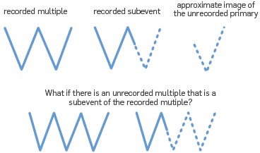
Figure 1 Using a recorded multiple to find an approximate image of an unrecorded primary of the multiple: illustrate the need to remove unrecorded multiples. A solid line () is a recorded event, and a dashed line (- - -) connotes an unrecorded event.
Hence, to image recorded primaries recorded multiples must first be removed, and to find an approximate image of an unrecorded primary requires unrecorded multiples to be removed.
The very use of multiples speaks to the primacy of primaries. Multiples are only useful if it contains as a subevent an unrecorded primary. A multiple that has all its subevents recorded has absolutely no use or value. All primaries are useful | and there is no substitute for a complete set of recorded primaries. Multiples can at times be useful, but are not in any sense the "new primary".
The recorded multiple event that can be used (at times) to find an approximate image of an unrecorded primary, must as an event be removed in order to image recorded primaries. The removing and using of multiples are always about our interest in primaries, both recorded and unrecorded primaries that we seek and require, and hence removing and using multiples are not adversarial, they serve the same single purpose and objective.
In the Executive Summary Presentation in the link there is a detailed discussion on this new perspective regarding removing and using multiples.
Here is the link with the executive summary video: http://mosrp.uh.edu/news/executive-summary-progress-2017.
Basically: (1) to image recorded primaries, with a smooth velocity model, recorded multiples must be removed and (2) for unrecorded primaries, to use a recorded multiple and a recorded subevent of the multiple to find an approximate image of an unrecorded primary subevent of the recorded multiple, any unrecorded multiple that is a subevent of the recorded multiple must be removed.
Hence, to image recorded primaries recorded multiples must be removed, and to find an approximate image of an unrecorded primary requires unrecorded multiples to be removed. The recorded multiple event that can be used (at times) to find an approximate image of an unrecorded primary must as an event be removed in order to image recorded primaries.
The key point is that it is primaries, both recorded and unrecorded primaries that we seek and require, and removing and using multiples are not adversarial, they serve the same single purpose and objective: the imaging of primaries. Multiples (recorded and unrecorded) need to be removed in order to image primaries (recorded and unrecorded, respectively).
If the multiple does not contain an unrecorded primary subevent, then is has no use. Whether or not an unrecorded primary is within the recorded multiple determines whether the recorded multiple is or is not useful. The use or lack of use of the multiple depends on whether or not a specific and particular primary has not been or has been recorded. What use is a multiple where all primary subevents of the multiple have been recorded. The answer: absolutely no use or value, none whatsoever the only interest for us in such a multiple is (as always) to remove that recorded multiple in order to not produce false, misleading and injurious images when migrating recorded primaries.
Hence multiples are NOT now rehabilitated events on equal footing with recorded primaries. They are NOT the new primaries and multiples are never migrated (That idea and thought of "migrating multiples" has no meaning. See [18], but as events themselves must always be removed. For those pursuing the use of multiples, it is of interest to know how unrecorded multiples will be removed.
The use of multiples is worthwhile to pursue, and to develop and deliver. Their value directly depends on the lack of adequate recorded primaries. There is no substitute for recorded primaries for the extraction of complex structural information and subsequent amplitude analysis. The high water mark of migration capability, Stolt CIII migration for heterogeneous media see e.g., [5], [10], requires recorded primaries. Methods that use a recorded multiple to obtain an approximate image of an unrecorded primary subevent, cannot achieve a Stolt CIII migration delivery and resolution effectiveness under any circumstances. The greatestdi_erential added-value [compared to all other migration methods] derives from Stolt CIII migration for complex structure determination and subsequent amplitude analysis, see [5], [11]. The priority of recorded primaries drives the priority of removing recorded multiples. In the next several sections we review the status, recent advances and open issues in removing multiples.
MULTIPLE REMOVAL: A BRIEF HISTORIC OVERVIEW AND UPDATE ON RECENT PROGRESS AND OPEN ISSUES
Multiple removal has a long history in seismic exploration. Among early and effective methods for removing multiples are CMP stacking, deconvolution, FK and Radon Filtering. These methods made assumptions about either: (1) the statistical, random and periodic nature of seismic events, (2) the ability to determine an accurate velocity model, (3) the assumed move-out differences between primaries and multiples, and (4) subsurface information including knowledge about the reflectors that generate the multiples.
However, as the industry trend moved to deep water and ever more complex offshore and on-shore plays, the assumptions behind those methods often could not be satisfied and therefore these methods were frequently unable to be effective and failed.
Methods that sought to avoid those limiting assumptions include SRME for free surface multiples and the distinct inverse scattering subseries (ISS) for removing free surface and internal multiples. SRME did not require subsurface information but only predicted the approximate time and approximate amplitude of first order free surface multiples at all offsets. In contrast, the ISS free surface multiple removal algorithm does not require subsurface information and predicts the exact time and exact amplitude of all orders of free surface multiples at all offsets. A quantitative comparison of SRME and the ISS free surface multiple elimination [ISS FSME] algorithm can be found in [19], [20]. That analysis helps to define when SRME and ISS free surface multiple elimination are the appropriate and indicated choice within the multiple removal seismic toolbox. SRME relies on an energy minimization adaptive subtraction to fill the gap between its amplitude and time prediction and the amplitude and time of the free surface multiple. That adaptive energy criteria assumes that there is less energy, in an interval of time, when a multiple is removed compared to when it is present. That assumption can and will fail for interfering or proximal events. The ISS free surface multiple elimination method does not require an adaptive energy subtraction, and, hence, is effective whether or not the multiple is isolated or if it is proximal or interfering with other events.
A key and central objective in multiple removal is not to damage target and reservoir primaries. For isolated free surface multiples SRME can at times be a reasonable tool box option. However, for free surface multiples that are proximal to (or interfering with other events), e.g., primaries, the ISS free surface multiple elimination algorithm is an important option and could be the appropriate and indicated choice. The ISS free surface multiple elimination requires the direct wave and source and receiver ghosts to be removed. Later in this paper, we will provide references that utilize variants of Green's theorem to remove the direct wave and ghosts, without damaging the reflection data.
The inverse scattering series internal multiple attenuation algorithm [6], [21], [22] is, at this time, the only internal multiple algorithm that does not require any subsurface information, no knowledge of the multiple generators and no seismic interpreter intervention. It is a multidimensional method that predicts the exact time and approximate amplitude of all internal multiples at all offsets. It is the current high water mark of internal multiple capability in the petroleum industry. In the sections below we review and exemplify the free surface and internal multiple removal status and describe recent advances in internal multiple elimination, and open issues.
THE ISS FSME AND SRME EQUATIONS
[6], [22] and[23] developed the multi-D ISS FSME algorithm from the Inverse Scattering Subseries for removing free-surface multiples (See Equations 1 and 2). For a 2D subsurface and towed streamer data, the ISS FSME algorithm for data without free surface multiples is

In Equations 1 and 2 D'1 is the input deghosted reflection data containing primaries, and free surface and internal multiples and D' is the output with primaries and only internal multiples. The quantities A(ω),ϵg and ϵs, in Equation 2 are the source signature, receiver depth and source depth, respectively; kg, ks are W Q wavenumbers of receivers and sources, ω is the temporal frequency and the obliquity 200 factor q is q=√(ω2/co 2) -k2).
The first term in this algorithm is the input data, D'1 in a 2D case, which is the Fourier transform of the deghosted prestack reflection data, with the direct wave and its ghost removed. The subsequent prediction terms, represented by D'2 , D'3 ,..., provide predictions of free-surface multiples of different orders. Specifically, each term in D'n (where n=2,3,4,...) performs two functions: (1) it predicts the nth order free-surface multiple and (2) it alters all higher order free-surface multiples to be prepared to be removed by higher-order D'j terms, where n=n+1,n+2,... The order of a free surface multiple is defined by the number of times the multiple has a downward reflection at the free surface.
The sum of these predictions (D 2'+D 3'+...+D n+1') provide free-surface-multiple predictions with accurate time and accurate amplitude (in opposite polarity) for free-surface multiples up to n-th order [6], [24].
The data, D' with free-surface multiples eliminated is obtained by Equation 1.
For the SRME approach, the method begins with the removal of: (1) the direct wave and (2) source and receiver ghosts, and then the SRME approximate free surface multiple prediction [25]- [27], M, can be expressed as follows

The input, P, is the prestack data for one temporal frequency, ω and where x g and x s are the location of the receivers and sources, respectively. Notice that, the input P for SRME and the input D 1 ' for ISS FSME are the same and both assume the removal of the direct wave and the source and receiver ghosts.
The output M in Equation 3 is the time and amplitude approximate free surface multiple prediction, provided within the approximations and assumptions in the SRME derivation and algorithm. The difference between the SRME approximate free surface multiple prediction, Equation 3 and the ISS exact free surface multiple predictor Equations 1 and 2 resides in the obliquity factor q, a function of frequency and wavenumber, and hence it causes an error in the SRME amplitude and phase prediction of the free surface multiple at all offsets. This SRME approximate free surface multiple is then energy minimization adaptive subtracted from the data in an attempt to match the amplitude and phase of the free surface multiple and thereby obtain the data without free-surface multiples. That lack of an accurate time and amplitude prediction in SRME is explicitly recognized by the energy minimization adaptive subtraction as a necessary and intrinsic part of the algorithm.
A quantitative comparison of SRME and the ISS Free Surface Multiple Elimination (FSME) algorithm can be found in [19], [20], see Figure 2 and 3. That analysis helps to define when SRME and ISS free surface elimination are the appropriate and indicated choice within the free-surface multiple removal seismic toolbox.
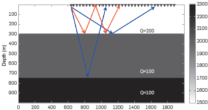
Figure 2 Model used to generated synthetic data. Two primaries (Blue) and one free-surface multiple (Red) are generated.
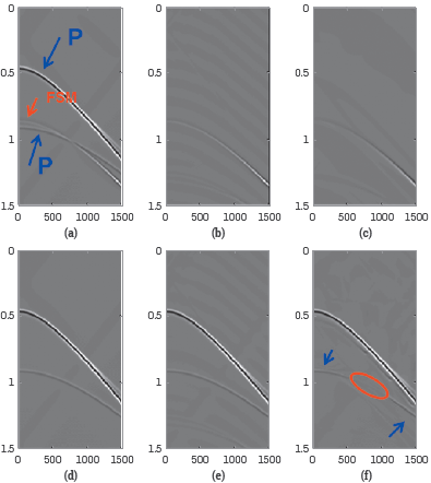
Figure 3 (a) Input data generated using model shown in Figure 2. Two primaries are pointed by the blue arrows, one free-surface multiple is pointed by the red arrow, (b) ISS free-surface multiple prediction (c) SRME free-surface multiple prediction (d) Actual primaries in the data (e) Result after ISS FSME (f) Result after SRME + Adaptive subtraction. The free-surface multiple is interfering with the recorded primary. The SRME + Adaptive damages the primary that interferes with the free surface multiple. The ISS free-surface algorithm effectively removes the free surface multiple without damaging the primary.
The result shows SRME + adaptive subtraction can be an effective and appropriate choice to remove isolated free-surface multiples, but can be injurious when applied to remove a FS multiple that is proximal or interfering with other events. The ISS FSME is effective and the appropriate choice whether or not the FS multiple is isolated or interfering with other events. The ISS FSME can surgically remove free-surface multiple that interfere with primaries or other events, and without damaging primaries.
There are many off-shore and on-shore plays where it is not clear, a priori, whether there are (or are not) free surface multiples that interfere with other events. The ISS free surface multiple eliminator is always a prudent choice.
THE CURRENT HIGH WATER MARK OF FREE SURFACE AND INTERNAL MULTIPLE REMOVAL
The ISS free surface multiple elimination algorithm (see e.g., [6], [22], [28]) predicts both the exact time and amplitude of all orders of free surface multiples at all offsets. It is effective with either isolated or interfering free surface multiples.
The ISS internal multiple attenuation algorithm attenuates internal multiples predicting the exact time and approximate amplitude of internal multiples is the only internal multiple algorithm that requires absolutely no subsurface information and often will be applied along with an energy minimization adaptive subtraction to remove an internal multiple that is not proximal to other events. To remove an internal multiple that is proximal to or interferes with other events (and therefore cannot rely on energy minimization, since the energy minimization criteria itself can fail under those circumstances), we need a more capable prediction, to surgically remove the multiple without damaging a nearby or interfering event. ISS internal multiple elimination had its origins in [29], discussion in [30], and an initial algorithm development in [31] and a fuller development and multidimensional algorithm in [32]- [34]
The ISS internal multiple attenuation algorithm is model type independent. That is, one absolutely unchanged algorithm (and with no change whatsoever in the computer code) predicts the precise time and approximate amplitude of all internal multiples independent of whether the subsurface is acoustic, elastic, anisotropic or anelastic. Filling the gap between the SS internal multiple attenuation and the elimination of the internal multiples is currently assuming an acoustic medium However a major contributor to the ISS internal multiple eliminator is the ISS internal multiple attenuator and the latter is model type independent. As we noted the gap filling part of the latter ISS internal multiple elimination algorithm [35] is based on an acoustic medium, and the effectiveness under different circumstances for acoustic, elastic and an-elastic media is evaluated in [34], [36] and [37]
THE ISS INTERNAL-MULTIPLE ATTENUATION ALGORITHM AND THE ID ISS INTERNAL MULTIPLE ELIMINATION ALGORITHM
The ISS internal-multiple attenuation algorithm was pioneered and developed in [21] and [22], The ID normal incidence version of the algorithm is presented in Equation 4 below (The 2D version is given in [6], [21] and [22] and the 3D version is a straightforward extension).
In Equation 4b 1 (z) is the constant velocity Stolt migration of the reflection data resulting from a ID normal incidence spike plane wave. ϵ1 and ϵ2 are two small positive numbers introduced to strictly maintain a lower-higher-lower relationship between the three water speed images and to avoid two water speed images at the same depth. b3 (k) is the predicted first order internal multiples in the vertical wavenumber domain. This algorithm can predict the correct time and approximate amplitude of all first-order internal multiples at once without any subsurface information.
Innanen and colleagues (e.g., [38]) have investigated the sensitivity of the choice of epsilon in Equation 4 in terms of the required lower higher lower pseudo depth relation that the subevents need to satisfy in order to combine to predict an internal multiple. They have suggested and have exemplified a non-stationary epsilon strategy, that navigate the issues between a too small (predictor becomes a "primary-like" artifact) and too large (missing predicting some internal multiples) epsilon value, and they propose that a priori geologic information can assist. Our view is that the very meaning of a primary and an internal multiple is a bandwidth dependent concept, and hence, e.g., there are events that we consider to be primaries that in fact under broader bandwidth would be a superposition of subresolution internal multiples. The ISS internal multiple attenuation and elimination algorithms assume definitions of primaries and internal multiples that are defined and have meaning within the bandwidth of the recorded data set.
The ISS internal-multiple attenuation algorithm automatically uses three primaries in the data to predict a first-order internal multiple. (Note that this algorithm is model type independent and it operates by taking into account all possible combinations of primaries that can be combined in a lower-higher-lower sense to predict internal multiples.).
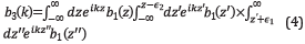
The following equations are the 1D pre-stack ISS internal multiple elimination algorithm, see [32] and [33] for details and 1D examples].
where
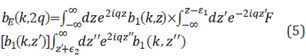
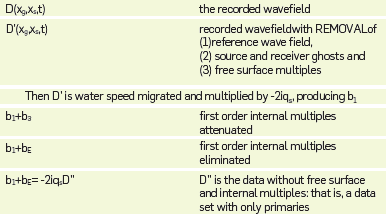
The data without internal multiples, D is provided by Equations 5-7 and b 1 +b E =-2iqD" (see the discussion later in this paper and Table 1 for details and a broader perspective on the processing chain and steps in multiple removal).
THE FIRST INVERSE-SCATTERING-SERIES INTERNAL MULTIPLE ELIMINATION METHOD FOR A MULTIDIMENSIONAL SUBSURFACE
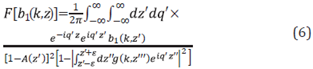
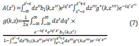
The multi-dimensional ISS internal multiple elimination algorithm, see e.g., [35], [39] is provided in Equations 8, 9 and 10. This elimination formula is for all first order internal multiples from all reflectors at once, and without subsurface information. A first order internal multiple has one downward reflection in its history.
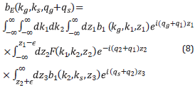
Similar to the 1D ISS internal multiple elimination algorithm [40] it is useful to introduce two intermediate functions F(k1,k2,z) and g(k 1 ,k 2 ,z) as follows:
Once again b 1 +b E =-2iqD", where D" is the data without first order internal multiples. The generalization for eliminating higher order internal multiples follows from the corresponding higher order ISS internal multiple attenuation algorithm in [6] and [21].
We thought that it might be useful at this point to remind ourselves of the data processing steps that towed streamer data goes through from the time it is recorded to the removal of all multiples and consists only of primaries. See Table 1.
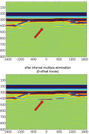
SYNTHETIC DATA EXAMPLE OF MULTI D INTERNAL MULTIPLE ELIMINATION
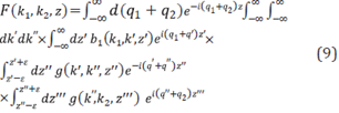
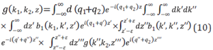
The left part of the Figure 4 shows the 2D model. The data is generated by a finite difference method. The acoustic model is designed so that the base salt primary is negatively interfering with a first order internal multiple whose downward reflection is at the water bottom.
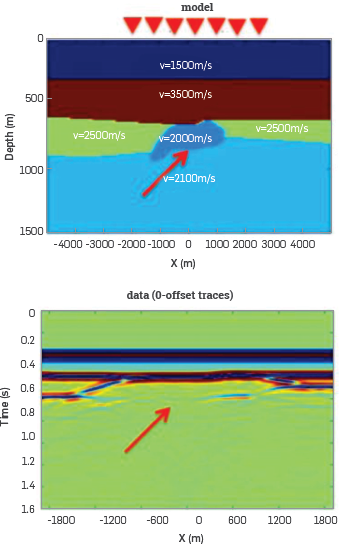
Figure 4 The model and zero offset traces of data. The base salt is almost invisible because the primary generated by the base salt is negatively interfering with an internal multiple.
The base salt is almost invisible because the primary from base salt is negatively interfering with the water bottom downward reflected internal multiple. The left hand side of Figure 5 shows that the ISS internal multiple attenuation plus energy minimization adaptive subtraction does not recover the base salt image. The right hand side of Figure 5 shows the result after ISS internal-multiple elimination, The base salt is recovered. It demonstrates that the elimination algorithm can predict both the correct time and amplitude and can eliminate internal multiples without damaging an interfering or proximal primary.
CONCLUSION ON INTERNAL MULTIPLE REMOVAL
The ISS multi-dimensional internal-multiple-elimination algorithm that removes internal multiples is one part of a three-pronged strategy that is a response to current seismic processing and interpretation challenge that occurs when primaries and internal multiples are proximal to and/or interfere with each other. That can frequently occur in on-shore and off-shore plays.
The other two parts of the three part strategy involve: (1) preprocessing for on-shore plays and (2) developing a new adaptive criteria for the internal multiple elimination algorithm. Recent progress in preprocessing non-horizontal undulating off-shore cables and on-shore acquisition can be found in the following references: [36], [41]- [50]. An example of a new adaptive criteria for the case of the ISS free surface elimination is provided in [1] We are pursuing a similar criteria (that derives as a property of the SS predictor) for internal multiple elimination.
The ISS internal multiple elimination is a direct solution for the removal of multiples within the assumed physics and acquisition requirements. The adaptive step is indirect and is designed for addressing the parts of reality and e.g. linear wave propagation assumption and acquisition limitations that are outside and beyond our assumed physics.
This new internal multiple elimination algorithm addresses the prediction shortcoming of the current most capable internal-multiple-removal method (ISS internal-multiple-attenuation algorithm plus adaptive subtraction). Meanwhile, this elimination algorithm retains the strengths of the ISS internal-multiple-attenuation algorithm that can predict all internal multiples at once and requiring no subsurface information. This ISS internal-multiple-elimination algorithm is more effective and more compute-intensive than the current industry-standard most capable internal-multiple-removal method, i.e., the ISS internal multiple attenuator. Within the three-pronged strategy, our plans include developing an alternative adaptive-subtraction criteria for internal-multiple elimination derived from, and always aligned with the ISS elimination algorithm. That would be analogous to the new adaptive criteria for free-surface-multiple removal proposed by [1], as a replacement for internal multiple elimination for the energy-minimization criteria for adaptive subtraction. We provide this new multi-dimensional internal-multiple-elimination method as a new internal-multiple-removal capability in the multiple-removal toolbox that can remove internal multiples that interfere with primaries without damaging the primary and without subsurface information.
Various strategies to provide an effective eliminator in anelastic media include: (1) developing a modeltype independent ISS internal multiple eliminator and (2) employ an ISS subseries that inputs data that has experienced absorption and dispersion and outputs the data as though it had only experienced an elastic subsurface, without knowing or needing to know or to estimate or determine the absorption and dispersion mechanism [13]
The capability and potential of the recently developed inverse scattering subseries that performs Q compensation without knowing, estimating or determining Q [13] and without low frequency or zero frequency data is illustrated in Figures 6, 7 and 8. The same ISS subseries that performs Q compensation without needing to know or determine Q, can be easily adjusted to provide a subsurface map of Q. That advance has implications in many seismic and non-seismic applications. Among applications are the ability to avoid the need for low and zero frequency data in all amplitude analysis methods, including all indirect model-matching and updating methods. There are very significant applications of this new Q compensation method to electromagnetic prospecting and data analysis. These two references [51] and [52] show how the role of Q in seismic wave propagation corresponds to conductivity in electromagnetic propagation. The latter represents the practical potential of producing a subsurface conductivity map, and therefore a way to distinguish water from oil in the surface.
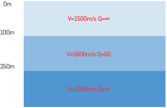
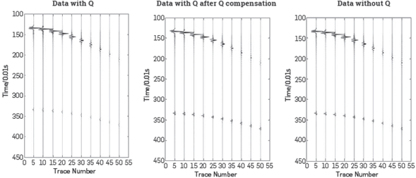
Figure 7 Left: Data generated by the model with Q. Middle: The data (with Q) after ISS Q compensation without Q Right: Data generated by the same model but without Q. [13].
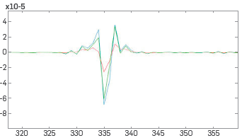
Figure 8 One trace comparison magnifying the event in the previous slide between 3.2 s -3.5 s. Red line: Data with Q. Green line: Data with Q after Q compensation. Blue line: Data without Q [34].
COMMENTS ON DIRECT INVERSION AND INDIRECT INVERSION (MODEL MATCHING):
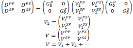
The only direct inverse methods for parameter estimation the parameter estimation subseries of the inverse scattering series, pioneered by [7], [53], [54], (see [5]) specify the data and algorithms. The required data is a complete set of shot records with multi-component primaries. In these references it is shown that the elastic inhomogeneous isotropic elastic wave equation becomes a matrix operator identity in terms of a data matrix (in 2D),
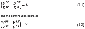
The inverse solution for V is a generalized Geometric series in the data matrix D, where the V PP , V PS , V SP and V SS contain the sought after mechanical properties of the subsurface.
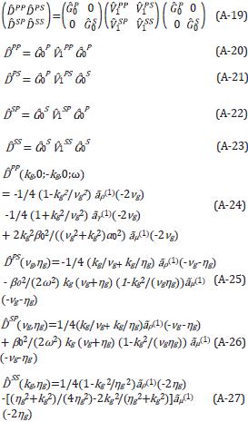
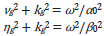
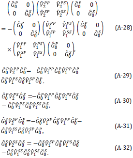
The forward series for D, in terms of V can be solved for one component of D, say, for example D PP. If one were to consider solving the latter forward problem for D PP in "an inverse sense", one would incorrectly deduce that D PP is an adequate data for an inverse solution. That thinking would violate the basic operator identity relationship (the Lippmann Schwinger equation) that solves for V (or any one component of V) in terms of the data matrix D. Please also see Appendix A for the detail relationship between D and V and why the entire data matrix D is required for a direct elastic parameter inversion, Equations A-28-A-32 and in addition a simple analytic example demonstrating that solving a forward problem in an inverse sense is not the same as solving the inverse problem directly.
In contrast, to the specificity in terms of data and inverse algorithms provided by direct solutions, with model matching methods, e.g., n the recent model matching approach, FWI there is no guide, no underlying theory or conceptual platform for what data is adequate, in principle, one trace, many traces, multi-component traces, and horizontal and vertical derivatives of displacement and pressure, and stress measurements and gravity data in fact, absolutely any data can be chosen to be model matched, including only one trace, or traces with only multiples. It seems reasonable that adding more data and data types would provide more constraints to search algorithms that might benefit and assist the parameter identification objective and reduce ill posedness however while including free surface multiples with primaries is often viewed as helpful, with added data constraints for the modeling to match, the addition of internal multiples seems in practice to be "too fuir model matching with too many complicated constraints to satisfy Under most circumstances internal multiples are attenuated before a FWI model matching begins. It seems that model matching with only primaries is viewed as not "full" enough, with primaries and free surface multiples that feels just right and perfectly full, and with the addition of internal multiples, apparently a little "too full", We are back to the lack of an underlying theory and framework, Why would a so called "full" wavefield inversion need to exclude internal multiples?
A great pedagogical advantage of indirect model methods is they are conceptually simple and readily understandable. Take a modeled trace and an actual trace and try to adjust the model parameters so the two traces match. Not hard to follow and understand. Indirect model matching methods also require a great deal of computer power and investment for search algorithms, and that expenditure "must" be based on a firm scientific foundation. In contrast, direct methods require an investment in understanding the physics and math-physics behind forward and inverse scattering. The first mention and derivation of the Lippmann Schwinger equation often has many in the audience dreaming of and pining for the simplicity of model matching concepts. Direct methods are often applied without any understanding of derivations behind the equations being coded and the services provided. For example, every major service company today and many oil companies provide a service based on the ISS internal multiple attenuator. It is extremely rare to find an individual who understands the underlying math-physics message and promise of the ISS series and how the ISS derives the isolated task subseries that attenuates internal multiples.
Indirect methods have a useful role and place within the seismic toolbox, and as with all seismic methods (including all migration, Green's theorem and ISS methods), we welcome and encourage a balanced view of the benefits, shortcomings and open issues.
CONCLUSION
Multiple removal and using multiples have one single exact goal: imaging primaries, recorded and unrecorded primaries. To be effective at reaching that objective recorded and unrecorded multiples must be removed. Since recorded primaries have the greatest potential (via Stolt CIII migration and migration-inversion and ISS depth imaging and inversion) for delivering structure and amplitude analysis, the removal of recorded multiples as a concomitant high priority and interest.
The confusion over "using" multiples is not a harmless misunderstanding without consequences because if multiples were in fact the new signal and the equivalent of primaries then we should no longer remove multiples, no more than we remove primaries that is the danger that derives from a misinformed premise and conclusion in thinking that removing and using multiples are adversarial.
In the history of useful methods and contributions that seek to accommodate limited data acquisition, like DMO, and 2D and 2.5D processing with asymptotic techniques in the cross line direction, eventually data acquisition advances to provide the data necessary to reach processing and interpretation goals and methods that seek to accommodate limited data become less interesting and less relevant.
Multiple removal is a permanent issue, whereas multiple usage is transient, and the latter will eventually be replaced by a more complete recording of primaries. In the interim, advances in both removing and using multiples are welcome and needed.