


 English (pdf)
 Article in xml format
 Article references
 Send this article by e-mail
 Cited by SciELO
  Cited by Google
  Similars in
SciELO
Similars in
SciELO  Similars in Google
 Permalink
1. INTRODUCTION
Seismic exploration of oil and gas in complex geological areas requires the development of techniques for the estimation of reliable velocity models, to generate a successful migration of seismic traces. Full waveform inversion (FWI) has been used to estimate high-resolution velocity models [1], and it reaches more detailed models than those attained by traditional inversion methods, as sparse-spike methods, recursive inversion, among others [2].
In marine seismic exploration, the Towed Streamer is the most widely used geometry, where one or more streamers containing the acquisition transducers are located to obtain the desired coverage. Another geometry used in marine acquisition, is the 2D Towed Streamer blended (blended geometry) [3]. It consists in a single cable or streamer that is dragged behind the exploration vessel together with various sound sources [4]. Subsurface reflections are below the line drawn by the movement of the vessel, resulting in a two-dimensional blended shot gather (horizontal and vertical).
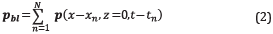
A blended shot gather involves temporary overlapping of multiple shots randomly located in the same acquisition. This is an emerging technology that reduces acquisition costs by decreasing the number of recorded shots, as it performs simultaneous source shooting (i.e. super-shot), as shown in Figure 1. It also decreases the number of times that the ship must pass through the traced path, thus reducing the seismic acquisition time and costs [5].
Most of the scientific community has focused its efforts on the de-blending stage, which is intended separate the blended sources to obtain non-overlapping shot-gathers using filters, deconvolution, muting, etc ... The generation of coded sources has been performed using only one encoding parameter such as time delay [5]; phase [6] or weight [7]. In those cases, the encoding process is associated with different probability distributions or empirical tests.
We present herein a formula for the acquisition of super-shots for FWI, without the de-blending stage. The encoding methodology is based on the minimum coherence problem and the estimation of the velocity models is performed via FWI, using blended data. Simulations and results are used to examine the proposed blending methodology from a practical point of view.
2. THEORETICAL FRAME
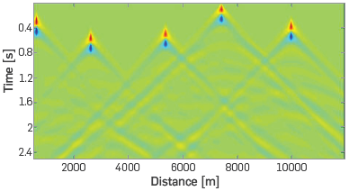
Blended data implies the acquisition of multiple shots at the same time (super-shot), producing an overlap between the traditional single shot-gathers. This overlap generates interference that affects the result of seismic approaches, such as FWI or seismic image migration.
A mathematical expression for a single shot, src, of the wavefield measured at the surface in the time domain can be obtained with the numerical solution of the 2D acoustic wave equation with constant density given by
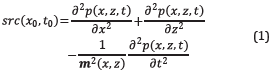
where, x and t are the spatial position and the time delay for the single source, respectively; m ϵR NxxNz (for the 2D case) is the acoustic velocity of the medium as a function of space location (x,z) and p is the scalar pressure field for different time steps, t. The observed blended data at the surface, p bl , is given by the linear sum of the N shots with encoding time delay, t n, and position, xn, as
where, tn∈Q t and x n∈Q x are the set of feasible values for both variables.
BLENDED CODED SOURCES
A blended data or super-shot p bt in terms of the pressure wavefield at the surface of a single shot located in the position x 0 and the time delay t 0, p(x-x 0,z=0,t-t 0 ), can be defined as the convolution (*) between the pressure wavefield and the matrix A, as

where A N ∈ R NxxNt is the binary coded matrix for each N super-shot as shown in Figure 2. The position and the rows represent the time delay when the source is activated. Each source is represented by one (1) in the coordinate (x n,t n). It should be noted that Equation 3 is equivalent to the expression in the Equation 2.
Figure 2 Physical representation of coded matrix A for one super-shot with five simultaneous sources, where the columns are the source position and the rows represent the time delay when the source is activated. The black cells indicate the activation moment of each source.
Each binary coded matrix A N is obtained distributing k sources within the super-shot with a minimum offset without overlapping between the intersection point of direct waves, (x p,t p), and the position of each source, as Figure 3 shows. The intersection point is defined as the crossing point of direct arrivals, which are propagated from source to receiver only in water. In real life, the water layer is known from the preliminary studies that delineate the acquisition trajectory and the type of vessel used.
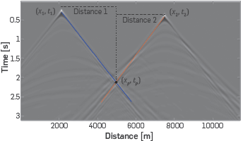
Figure 3 Representation of the intersection point (xp,tp), with the cross point between the direct wave of first shot (blue line) and the direct wave of second shot (red line). The distance between the position of each source and the intersection point (distance 1 and distance 2) is compared with the minimal offset clear for determine if this distribution fixes.
Direct waves are modeled using the equations for ray tracing in laterally homogeneous Earth models [8]. Being the ray parameter p defined as

where u=1/v is the slowness, with v as the velocity of the layer and θ is the ray incidence angle (from vertical). The expression for the surface-to-surface travel time T(p) and the total distance X(p) for a constant layer are,
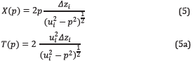
being Δz( the thickness of the layer, in this case the water layer.
Encoding N blended shots require to optimize each coded matrix A ¡ with the aim to each one acquires data from different areas. Each matrix A¡ ∈ R NAX1 becomes a column of matrix B ∈ R NAXN with N A =N x - N t as shown in Figure 4. An optimal coding is obtained finding the minimal mutual coherence between the columns of the design matrix B. The minimal mutual coherence implies linearly independent columns of the design matrix B, which involve different coded matrices with the least interference between super-shots.
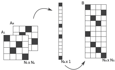
Figure 4 Process to generate the design matrix B where each column is the vectorization of matrix Ai.
The mutual coherence of matrix B is the largest absolute normalized inner product between different columns of B [9], and it is given by
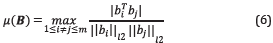
where b ¡ is the i-th column of B, being each b ¡ column function of the variables x n and t n .
The minimization problem of mutual coherence of the design matrix B as

To simplify the problem, the modification of the optimization problem showed by Obermeier [10] can be used. It is possible to use only the upper triangular components of the matrix U=B TxB to compute the mutual coherence, where the elements of the upper and lower triangular matrix are the same, Equation 8.
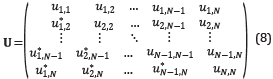
The matrix U can be expressed as the vector u=(u 1,2,u 1,3,…,u 1,N,u 2,3,…,u N-1,N) to compactly represent these elements. We use the notation u ij to represent the element in the vector u that corresponds to the value of U at the location (i,j) and the definition of f(x n,t n) is expanded as follows:

Where f i (xn ,t n) computes the i-th column of B.
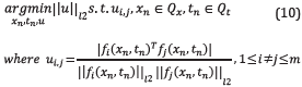
With these modifications, the equivalent mutual coherence minimization problem can be formulated as
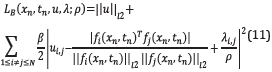
This optimization problem can be formulated without constraints using the Augmented Lagrangian method with equality constraints [11],
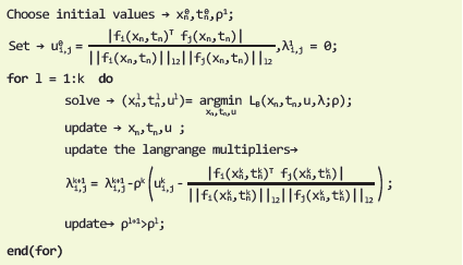
The coherence minimization procedure is summarized in Algorithm 1 (see Table 1).
The minimization problem, with Obermeier modification [10], can be seen as to diagonalize the matrix U=BT×B that contains non-zero values outside the diagonal in a diagonal matrix, as shown is Figure 5. Where the numerical value of the diagonal elements represents the number of simultaneous shots with different codification within each super-shot and the absence of values outside the diagonal represents a zero correlation between super-shots, that is, a source distribution where the encoding parameters are different in each super-shot and, in turn, they are different with respect to the rest of the shots.
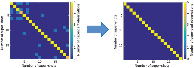
Figure 5 Representation of the minimization problem to diagonalize the initial matrix U in a diagonal matrix. The final matrix U represents 20 super-shots and 5 simultaneous sources within each super-shot. The diagonal represents 5 different coded sources in each super-shot and the zero values in the triangular matrix a zero correlation with each acquisition source.
FULL WAVEFORM INVERSION
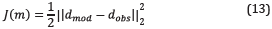
Full Waveform Inversion (FWI) is a processing tool that estimates the subsurface parameters from an initial model and the acquired data at the surface. FWI updates the model by decreasing iteratively the misfit function given by the squared l 2-error norm between the acquired data, d obs, and the modeled data, d mod .
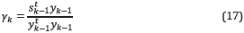
The misfit function [12] is given by 1 2
It can be minimized using a gradient descent method [1] by updating iteratively the velocity model as
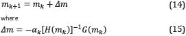
being Δm the search direction where G(m k) is the gradient that represents the evolution direction in the misfit function, H(m k) is the Hessian, which represents the magnitude of this direction, both evaluated at mk and αk is a scalar step length value.
The velocity gradient for the 2D acoustic and isotropic wave equation is computed using the first order adjoint state method by [13]
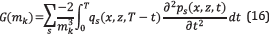
where T is the recorded time and t is the time variable, p s is the forward wavefield generated by the source src(x,z); q s is the backward pressure wavefield generated by the residual data (the difference between the modelled and acquired data); s represents a specific shot; each shot produces its own gradient and therefore, the final gradient per iteration is the summation of all the gradients.
The Hessian matrix is not directly computed, but an approximation of the product between the inverse of the Hessian matrix and the gradient ([H(v k)] -1 g(v k)) using L-BFGS method was defined by Liu and Nocedal [14]. This approximation uses the last n gradients and velocity models to compute the step forward and it needs at least two gradients and two velocity models to obtain an approximation of the search direction Δm=r.
Algorithm 2 (see Table 2) shows the pseudocode of this method, where s
k
=m
k+1
-m
k
,y
k
=g
k+1
-g
k and σk=1 /  s
k. The matrix
s
k. The matrix  is approximated by a diagonal
  =y
k
l, with
=y
k
l, with
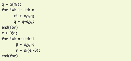
The step length factor is set to αk=1, and the condition

is tested, where J(m k) is the misfit value obtained from the wavefield propagation in the velocity model m k at the kth iteration and J(m k+1) is the misfit value obtained with the updated velocity model given by the L-BFGS method.
When the condition given in Equation 18 does not hold, then the step length αk decreases by half until the condition is satisfied.
Blended data implies that in the FWI methodology the number of observed data is less than the number used traditional implementation, where we acquire each shot individually. This represents the FWI method less gradient computation (Equation 16), which decreases the processing time by making fewer calculations.
3. EXPERIMENTAL DEVELOPMENT
The Ricker wavelet was used to generate both, the observed data and the modeled data at each FWI iteration. The mathematical expression used to obtain the source is

where f is the central frequency, t is the time window and t 0 is a time delay.
The FWI multiscale approach is a strategy that allows to first recover the background of the velocity model and then go detailing the structures using an inversion in which a sweep of the central frequency of the wavelet is made from low frequencies to higher frequencies. For our experiments, the first central frequency is 3[Hz] [15].
On the implementation, the Finite Difference in Time Domain method (FDTD) is used to discretize the wave equation. The time and spatial discretization use a second order and eight order stencils, respectively. The CPML zone uses 20 points.
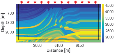
The Marmousi velocity model that was created in 1988 by the Institut Francais du Pétrole (IFP), is based on a profile through the North Quenguela trough in the Cuanza Basin in Angola and it contains many reflectors, steep dips and strong velocity gradients in both vertical and lateral directions [16].
It used a Marmousi model with a distance of 9.2 km and a depth of 3km on a grid of 25 meters discretized in a grid of 368x120 points (see Figure 6a) and a minimum offset of 750[m] of data without overlapping; the maximum number of simultaneous sources within the super-shot is 5.
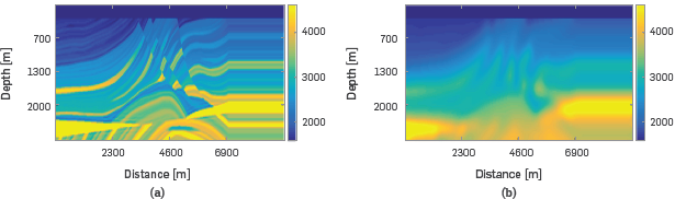
Figure 6 (a) Marmousi model size 9.2km x 3km as an original velocity model, (b) Marmousi smooth model size 9.2km x 3 km as an initial velocity model.
Three different sets of sources are generated: twenty coded super-shots with 5 simultaneous sources using the optimal coded implementation proposed in this paper; twenty randomly coded super-shots with 5 simultaneous sources; and 100 equally spaced traditional sources equivalent to the twenty blended sources. All of them with 328 receivers spaced evenly in the acquisition area
The performance of the three different source distributions in the FWI is measured using the processing time and the PSNR value of the obtained velocity model against the real model using the different source distributions. PSNR allows quantifying the quality of the velocity model Figure 6b comparing this with the original velocity model.
Other important parameters of the experiments are shown in Table 3.
Table 3 Main parameters of FWI used to run the experiments.
| Parameter | Value | |
|---|---|---|
| Model Distance | 368 [pt.] | |
| Model Depth | 120 [pt.] | |
| Grid spacing | 25 [m] | |
| Time step | l[ms] | |
| Recording time | 2[s] | |
| Number of sources | 100 | |
| Number of receivers 828 | ||
| Size of absorbing boundaries | 20 [pt.] | |
| Number of frequency steps | 3, 6 and 9 Hz | |
| Number of iterations per frequency | 20 | |
MUTUAL COHERENCE MINIMIZATION
For the case study, 20 initial random coded matrices are generated (matrix A 1 to A 20) where the plausible range of data for the encoding of the parameters is: Q T ∈[0.1,0.7] seconds, with a time step of 1[ms] and Q x ∈[21,347] points with a spatial step of 1 point.
It generated 20 coded matrices A of size 340x70 with 5 simultaneous inner sources. By vectorizing each encoding matrix as a column of the design matrix B, we obtain a design matrix B of size 20x23800 Being the initial U matrix used for the minimization problem Equation 8, U= B T B of size 20x20.
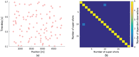
Figure 7a represents the initial random coded of each source, where the X-axis is the horizontal position of each source and the Y-axis the time delay. The initial code of sources have large empty areas highlighted in red and areas of sources agglomeration marked in blue, where more than one source has the same code. These problems in the initial code are represented in the matrix U Figure 7b, where values in the diagonal other than 5 mean that there is at Least one source with the same code, super-shot 4 and 20, and nonzero values in the triangular matrices shows dependent observations between super-shots, i.e. shots with equal codes.
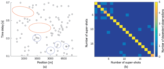
Figure 7 (a) Representation of initial random code of each source, areas highlighted in red presents large empty areas without sources and blue areas represent an agglomeration of sources, (b) initial matrix Û for the minimization problem μ(B)=0.78.
Starting from the random matrix U, the mutual coherence for the initial distribution of sources is μ(B)=0.78, obtaining after 25 Iterations a coherence of μ(B)=0.12.
Figure 8a represents the final code of each source, where a more homogeneous distribution of sources is observed. Figure 8b, presents the final U matrix where the diagonal takes the expected value of 5, showing that each super-shot has 5 different simultaneous shots; the reduction of non-zero values in the triangular shows the improvement in the encoding distribution of sources.
TRADITIONAL DISTRIBUTION
For the traditional distribution of sources, the 100 sources are Located equally spaced in the acquisition area (inner square area Figure 9, where the borders are the CPML absorbing zone of 20 points), each source (red starts in Figure 9) is activated and acquired individually obtaining 160 observed data. There are 328 receivers equally spaced with 160 sources placed every 75 [m].
RANDOM BLENDED DISTRIBUTION
For the random blended source distribution, 20 super-shots within 5 simultaneous sources are located in the acquisition area with 20 points of CPML absorbing zone, Figure 10 shows an example of the distribution of 3 of the super-shots, where we can see that some sources of each super-shot are the same for other super-shot (source 1 of super-shot 1 and 2 and source 5 of super-shot 2 and source 4 of super shot 3).
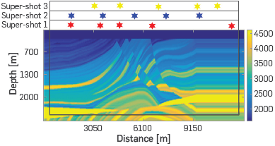
Figure 10 Representation of three Random Blended distribution of super-shots as red stars, for the first super-shot; blue starts, for the second one; and orange starts for the third one. The code for each super-shot is obtained using a random uniform distribution for the spatial parameter and Random Gaussian distribution for the time delay parameter. Along the acquisition area (inner area of the figure), with 20 points of CPML frontier (black borders of the figure).
The codification is obtained using a random uniform distribution in the spatial parameter, and random Gaussian distribution for the time delay parameter. There are 328 receivers ,equally spaced, and the minimum and maximum values of separation between sources are 25 [m] and 6525[m], respectively.
OPTIMAL CODED BLENDED DISTRIBUTION
For optimal blended distribution of sources, 20 super-shots within 5 simultaneous sources are in the acquisition area with 20 points of CPML frontier producing 20 observed data sets, obtaining the codification with the methodology proposed hereunder. Figure 11 shows an example of the distribution of 3 of the super-shots, where each acquired data from different areas. There are 328 equally spaced receivers and the minimum and maximum value of separation between sources are 750 [m] and 3225[m] respectively.
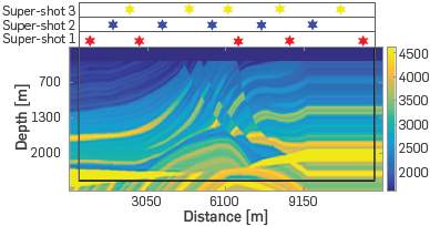
Figure 11 Representation of three Optimal Blended distribution of super-shots as red stars, for the first super-shot; blue starts, for the second one; and orange starts for the third one. The code for each super-shot is obtained using the methodology proposed in this document, along the acquisition area (inner area of the figure), with 20 points of CPML frontier (black borders of the figure).
4. RESULTS ANALYSIS
To compare the FWI algorithm for traditional, random blended distribution, and optimal blended distribution proposed in the document, three frequencies are used during the inversion 3, 6 and 9 [Hz], the number of iterations per frequency is set to 20, and the propagation time is set to 2 sec. The initial velocity model is depicted in Figure 5b, which is a smoothed version of the original Canadian model Figure 5a.
For each of the three experiments explained in the last section, we started with the smooth Marmousi velocity model (Figure 5b) as the initial velocity model in the first step of frequency for the multiscale FWI. Figure 12 shows the results of 20 iterations using the three different distributions of sources. Figure 12a, traditional distribution of sources, Figure 13b, random blended distribution of sources and Figure 12c optimal blended distribution proposed in the document.
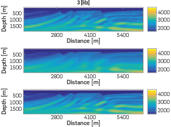
Figure 12 Final velocity models for the first stage (central frequency 3 Hz) in the multiscale FWI, using the smooth Canadian model, Figure (5b) as initial velocity model, and the three sets of observed data. Figure (a) Velocity model with a traditional distribution of sources, (b) Velocity model with a randomly blended distribution of sources and (c) Velocity model with an optimal blended distribution of sources.
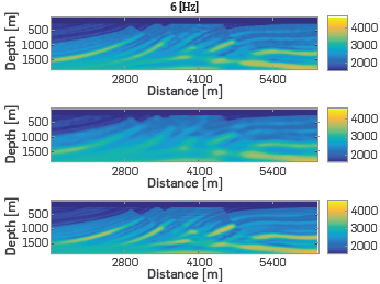
Figure 13 Final velocity models for the second stage (central frequency of 6 Hz) in the multiscale FWI, using for each experiment the final velocity model of the previous frequency step shown in Figure 9 as initial velocity model, and the three sets of observed data. Figure (a) Velocity model with a traditional distribution of sources, (b) Velocity model with a randomly blended distribution of sources, and (c) Velocity model with an optimal blended distribution of sources.
The optimal blended distribution shows a better delimitation of the first velocity zone of 4000 [m/s] than the random blended distribution (yellow zones in Figure 12b and Figure 9a). Being the PSNR value at least 2[dB] upper in the optimal distribution than the random distribution.
For the next frequency step (6 Hz), the initial velocity models for each experiment corresponds to the final velocity model of the previous frequency step shown in Figure 12, using the three different distributions of sources. Figure 13a, traditional distribution of sources, Figure 13b, random blended distribution of sources and Figure 13c optimal blended distribution proposed in the document. Final velocity models of the traditional and optimal distribution of sources look similar, being the PSNR value a metric to determine how close to our real model each one is, as presented in the second Line of Table 4. It may be observed that final velocity models with the optimal blended acquisition, Figure 14c, presents artifacts near the borders. The random blended distribution of sources generates Less defined structures backed up with the lower PSNR value.
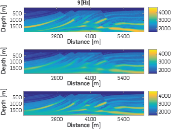
Figure 14 Final velocity models for the second step of frequency, 9 Hz, in the multiscale FWI, using for each experiment the final velocity model of the previous frequency step shown in Figure 10 as initial velocity model, and the three sets of observed data. Figure (a) Velocity model with a traditional source distribution, (b) Velocity model with a randomly blended source distribution, and (c) Velocity model with an optimal blended source distribution.
Table 4 PSNR for the multiscale FWI approach using a different distribution of sources.
| Freq. [Hz] | Traditional PSNR | Random Code PSNR | Optimal code PSNR |
|---|---|---|---|
| 3 | 26.06[dB] | 24.47[dB] | 25.63 [dB] |
| 6 | 27.58[dB] | 25.48[dB] | 27.12[dB] |
| 9 | 28.97[dB] | 26.63[dB] | 28.33[dB] |
For the last step of frequency (9 Hz), the initial velocity models for each experiment corresponds to the final velocity model of the previous frequency step shown in Figure 13, using the three different source distributions. Figure 14a, traditional source distribution Figure 14b, random blended distribution of sources and Figure 14c optimal blended distribution proposed in the document.
The third line of Table 4 shows the PSNR value for the last frequency step, and the traditional distribution is the model with the highest PSNR value as each source is acquired individually without interference of the others. However, this type of acquisition requires the ship passing more times through the exploration area and therefore, being more expensive than the proposed methodology that acquires more of one source simultaneously. The proposed codification reduces the processing time in the computation of FWI 5.23 times with traditional FWI, obtaining a final velocity model with a PSNR value higher than the random distribution.
The optimal blended distribution obtains in the first frequency step (3[Hzj) a PSNR value closer than the PSRN of random blended distribution in the second step (6[Hz]). This behavior continues in the next pair of frequency, 6[Hz] for optimal blended distribution and 9[Hz] for random blended distribution.
Figure 15 shows the evolution of each experiment comparing the execution time versus the PSNR value of each distribution of sources and each frequency step. Being traditional distribution (green marks), random blended distribution (red marks) and optimal blended distribution (blue marks). We use three different figures to show each frequency step, squares, diamonds and circles for 3 [Hz] 6[Hz] and 9[Hz] respectively.
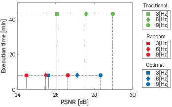
Figure 15 Execution time per frequency step versus PSNR of each velocity models, with squares being the first frequency step (3[Hz], diamonds the second frequency step (6[Hz]) and circles the last frequency step (9[Hz]). Each color represents one of the three experiments, traditional distribution of sources, (green), random blended distribution of sources (red), and optimal blended distribution of sources (blue).
The execution time for each frequency step, in the three experiments, Is approximately the same, being 8.32 [min] for both blended FWI (random and optimal) and 43.40[min] for the traditional case.
The progression can be observed in a better velocity model (with higher PSNR value) of each frequency step, it being the best velocity model obtained by traditional source distribution (green marks), followed closely by Optimal Blended distribution (blue marks) where the difference between traditional PSNR and optimal PSNR value for each frequency decreases in every frequency step, with a final difference of 0.6 [dB].
The optimal blended distribution obtains in the first frequency step (3[Hz]) a PSNR value closer than the PSRN of random blended distribution in the second step (6[Hz]). This behavior continues in the next pair of frequency, 6[Hz] for optimal blended distribution and 9[Hz] for random blended distribution.
CONCLUSIONS
In this work, a methodology for optimal coded blended sources has been presented with the aim of improving the results of 2D blended FWI in contrast to the randomly coded blended sources and the traditional equally spaced sources.
The minimization problem developed can be seen to diagonalize an initial matrix U that contains non-zero values outside the diagonal in a diagonal matrix, where the numerical value of the elements of the diagonal represents the number of simultaneous shots with different codification within each super-shot and the absence of values outside the diagonal represents a zero correlation between super-shots, that is, a distribution of sources in which the encoding parameters are different in each super-shot, and in turn they are different with respect to the rest of the shots.
The methodology improves the final velocity model, which is closer to the model obtained with the traditional acquisition, with a difference of about 0.6[dB], in contrast to the 2[dB] obtained by the randomly blended sources. Furthermore, the processing time is the same for the two blended FWI with an acceleration of near 5.23 times in computation time if both are compared with the traditional FWI. Optimal blended distribution obtains a balance between less processing time and quality of the image with a higher PSNR value than random blended distribution, observed in Figure 15, where the difference between the PSNR value of traditional and optimal blended distribution is lower in each frequency step.
Blended data implies that in the FWI methodology the number of observed data is less than that used in the traditional implementation, where we acquire each shot individually. This represents in the FWI method less gradient computation, which reduces the processing time by making fewer calculations.
Traditional acquisition produces a better velocity model after the FWI process, but it requires one image for each source increasing the acquisition time, the number of times that the vessel goes through the exploration trajectory, increasing the acquisition cost. The processing time is higher than blended FWI due to it is need of calculating more velocity gradients.
FUTURE WORK
It is necessary to analyze the effect of blended acquisition interference with other measures to quantify the difference of data sets in a real scenario. PSNR is only plausible in a synthetic case, where we know the original velocity model. In a real case cycle skipping of traces could be used as quality control, which measures the similarity as a function of the displacement of one trace relative to the other.

