


 Inglês (pdf)
 Artigo em XML
 Referências do artigo
 Enviar este artigo por email
 Citado por SciELO
  Citado por Google
  Similares em
SciELO
Similares em
SciELO  Similares em Google
 Permalink
1. INTRODUCTION
Modeling wave propagation in real sub-surface is a complex task: the detailed propagation physics is complicated and several simplifying approximations are required for computing the solution for many practical situations. For example, it is usual to ignore the effects of attenuation in wave propagation; however in real life, the earth exhibits elastic and viscous behavior, properties that must be considered when one is interested in real and detailed physical processes associated, for example, with wave propagation in the subsurface for seismic exploration.
Ignoring any viscous or elastic behavior in the medium leads to the so-called acoustic wave propagation. Although unrealistic, in general, it is the simplest (but often practical) modeling approximation. Together with the assumption of isotropy, acoustic wave propagation has been widely used in different situations in seismic exploration [1]- [4]. However, to obtain accurate data on the physical properties of the sub-surface in realistic situations, the acoustic wave approximation does not provide any further information and it becomes necessary to do a better modeling of the propagation of waves. In particular, the realistic modeling of wave propagation is an important step in earth subsurface imaging process.
A step forward in the direction of doing realistic modeling of wave propagation is to consider the effects of viscosity. The visco-acoustic media can be defined as a medium without cross propagation, although it exhibits attenuation in the amplitude of the longitudinal wave. This medium presents two phenomena, dissipation and dispersion. The first one is produced by energy absorption such that the amplitude of the wave is reduced especially at high frequencies, while the second is induced by the change in the refractive properties of the media, where the wave velocity depends on the frequency [5].
To describe the attenuation of energy in the seismic wave front [6] proposed a model based on linear solid material rheology and memory variables. Later, [7] followed the same modeling approach, using, however, only one relaxation mechanism. They show how the method works to compensate for attenuation in least-squares reverse time migration. [8] used a visco-acoustic wave equation to compensate for the energy decrease of wave propagation in a realistic media, using an extrapolator based on the propagator of the wave equation in the forward and backward direction. Visco-acoustic modeling has been implemented also in 3D high computing demand simulations [9], [10] and has also been used in the development of specific geometrical configurations (TTI) [11], exhibiting accurate descriptions of the wave propagation in the media.
In general, visco-acoustic phenomena are modeled explicitly as frequency-dependent functions. The solution of the visco-acoustic wave equation in frequency domain must be performed numerically, and because of its simplicity and computational efficiency, the usual approach to solve it is to use finite difference methods. Nevertheless, the propagation problem must take in to account, besides the complex nature of the differential equation, crucial ingredients such as the source term and boundary conditions [12], [13].
In frequency domain, spatial resolution changes every time frequency changes, which complicates the characterization of different parts of the model such as the size of the zones of boundary and the size of the seismic source. All of the foregoing makes solutions of the visco-acoustic wave equation in frequency domain a problem far from trivial. In particular, since at a given frequency the structure of the grid should adapt to the scales associated with the frequency, the energy injection in the media could be radiated at different scales if not considering these effects carefully. The distribution of such energy among grid cells close to the source is a topic that is poorly discussed in the literature, especially the discretization of the source, which is commonly modeled as a Dirac delta function to describe its spatial part, [14]- [16]. This turns to be key in the solution of the numerical forward problem.
The same occurs with boundary conditions: Sponge absorbing boundary condition (ABS) Convolution Perfectly-matched layer (CPML), Perfectly-matched layer (PML), all having parameters that must be tuned, as can be observed in [18], [20] and [21].
When solving the problem of wave propagation in time domain, these are probably easy to fix, but in frequency domain, they are problematic, once again because the size of the region where absorbing boundaries work change with frequency and with the way attenuation is being modeled at the boundary. For example, in [17], these parameters are chosen based on trial and error. How to deal with these parameters? We present in this paper a study of how to deal with PML boundary conditions in frequency domain, showing in particular how to model, implement and control the behavior of the seismic source, and how to estimate the values of the parameters that control the behavior of this model. Furthermore, we show practical functions that allows the determination of the parameters required to model the performance of the PML boundary conditions.
For approaching this analysis, we used the following structure: First, in section 2 we present the basic theoretical considerations relative to our problem, presenting the basic equation used to model visco-acoustic wave propagation. Then, we present some considerations on the source term for seismic wave propagation, as well as considerations associated with the modeling of PML boundary conditions. Then, in section 3, we discuss the results obtained from the modeling of the source term and PML; finally, in section 4 we present our conclusions.
2. THEORETICAL FRAME
THE SOURCE
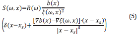
We consider the propagation of waves in 2D for the case of a visco-acoustic media. For this purpose, the equation for wave propagation in our visco-acoustic medium can be expressed as [16]
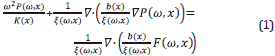
where P is the pressure field, K is the acoustic bulk modulus, ξ is the damping function [6] and b is the inverse of the medium density.
There are several choices on how to model attenuation. For example, using the models described in [5], which defines the wavenumber as K(ω)=ω/c(ω)=ω/v(ω) -ic(ω), where c(ω) is the complex velocity, v(ω) the phase velocity and k(ω) the attenuation wavenumber, one can rewrite things in terms of ξ like
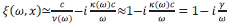
Where y is the rate deformation function related to the viscosity of the medium that is often related to the Q attenuation factor, which in the simplest case (Kolsky model, see e.g. 5) is y/ω=1/2Q.

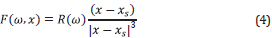
such that F(ω,x) is a body force. The source in these models is generally an impulse at point x s =(x s ,z s). The Ricker wavelet is a possibility to represent a seismic source, such that ∇ , F(ω,x)=R(ω)δ(x-x sJ where R(ω) is the Ricker wavelet given by
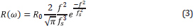
where δ(x-x s) is a Dirac delta function, but in the discretized domain can be represented with the Kronecker delta. The R 0 is the maximum amplitude of the ricker wavelet and f s is the principal frequency of the source. Now, assuming that the divergence of the force is ∇ , F(ω,x)=R(ω)δ(x-x s), the force could be expressed as
Thus, and using Eq. (1), we can write
Here, one can safely discard the second term to the right. When the velocity, density and attenuation are not constant, we propose for the source
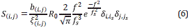
Where (i s ,js) is a point in the grid where the source is placed and δi,isδj,js can be approximated as
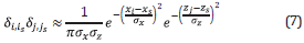
This approximation comes from the Dirac delta function as the limit (in the sense of distributions) of the sequence of zero-centered normal distributions δσ(x)=1/(√πσ)exp-(x/σ)2 as →0. The factor σ must have a relationship with the grid spacing, i.e. σx= σz~ Δ.
The discretization of the Dirac delta is used because of the changes in grid spacing, which according to the condition Δ=λ/G r =c min /(fG r) depends on the frequency. It is important to make sure that the energy source is distributed evenly within the space to avoid losses by locating the entire amplitude at a point that cannot be located unequivocally in all grids. Therefore, it must meet the property of the Dirac Delta in the discrete case.
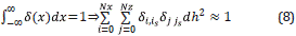
On such basis, it may be stated that the solution, is well defined in the discrete domain [14], [15]. Thus, we can define a=ax=az as, using Equation 7:
where s is a parameter that must be tuned to make sure that condition (9) is fulfilled, and at the end the parameter used to control the energy distribution of the source in the model.
PERFECTLY-MATCHED LAYER (PML) ABSORBING BOUNDARY CONDITIONS
Another important ingredient for the solution of Equation 1 is the boundary condition. In this work, we will study the use of perfectly-matched absorbing boundary conditions (PML). The absorbing boundary condition is a virtual boundary, very simple to use, as our media is dissipative in principle.
The PML method consists on using two damping functions to suppress the value of the pressure field in the boundaries at the edges of the square computational domain, yx(x) and y z (z) and a non-physical pressure wavefield P x and P z such that P=P x +P z . This technique is similar to a sponge-like absorbing boundary condition [18], but attenuation occurs at each dimension independently. The effect of these absorbing boundary conditions is that waves propagate in the medium, resembling the behavior of waves that propagate in an infinite medium (no reflections are produced at the borders of the computational domain), such that no need for any particular boundary conditions are required to specify the structure of the solution.
We simply expanded the computational domain ℧ with size characterized by N x xN z to the expanded domain ∂℧ with size N xe xN ze where N Xe =N x +2n xpm l and N ze =N z +2n zpml, where n xpml and n xpml are the number of extra points for the boundary condition (see Figure 1). In the expanded region, the damping functions have the form [17].
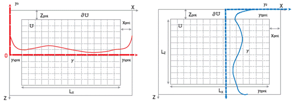
Where y(ω,x,L z) is the rate deformation function related to the viscosity of the medium introduced a few equations ago, which we will assume as a constant parameter. Note that the functions y zpml (ω,x) and y xpmi (ω,x) are modified deformation functions that apply only in the region of the extended domain. However, the idea is that these deformation functions should be coupled with the deformation functions (and, therefore, to the attenuation) in the original field ℧. Here, m 0 is a parameter that should depend on the frequency and takes a value that makes the amplitude of the wave at the boundary of the domain to fall below a given threshold.
As to the corners, which generate well-known edge problems [17], we use the conventional treatment of averaging the boundary conditions at x and z [22].
Once again, for a given form of the damping function (ω,x,L z) , the parameter m 0 controls the behavior of the PML. We show how this parameter depends on frequency and find a way to fix his value in our implementation of the visco-acoustic modeler. It should be noted that the behavior of the PML also depends on the value of the number of pixels one considers to extend the domain, N xe ,N ze . If these numbers are too small, waves going through the PML region will not attenuate completely, thus producing artificial reflections on the computational domain. Furthermore, if one uses N xe ,N ze that are too large, the attenuation will take place, but there will be a waste of computational resources trying to solve the problem of wave propagation in regions that are of no interest. It would be good to then find a way to identify the smaller values of Nxe ,N ze to make sure that the behavior of the PML is the right one.
3. RESULTS
Now, we discuss the result of our exploration. First, we show how we use Equation 9 to study the effects of our model for implementing the seismic source and controlling its behavior through the use of parameter s. Then, we show how we control the behavior of the PML boundary through parameter m 0 .
Specific details on how we solve the differential equation using a mixed grid are out of the scope of this work, but r the reader may refer to [16] and [19] for more details on its implementation.
THE SOURCE TERM
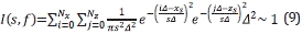
To get a correct value for s, we calculate Eq. (9) for different frequency values, assuming the position of the source is x s=1Km and z s=1Km in a field of area of 2Km x 2Km, with c=2100 m/s. The frequencies we used are f=1,5,15,30,50Hz. We do not compute it for higher frequencies as the Δ in these cases is smaller, approaching the continuous form of the Dirac delta. With these values, we reach Figure 2.
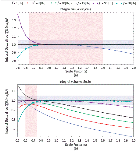
Figure 2 (a) Integral values for discrete Dirac delta calculate for equation 9 for different frequency values, assuming the position of the source is Xs = 1 Km and Zs = 1 Km; (b) Placed at Xs = 1 Km and Zs = 0.015 Km.
As we can see in Figure 2a, the values of l(s) remain close to 1 for s>0.9, except for the solution at f=lHz. However, in order to not being too restrictive, we notice that for scales in the range s=[0.65,1.6] l(s) keeps constrained in the range [0.95,1.05], It could be argued that it is enough to ensure the conservation of properties of the delta function around the source. For s (s<0.95) smaller value, the discretization affects the estimation of the spread of the source significantly.
In Figure 2b, we do the same calculation but with the source placed at x s=1Km and z s=15m. We can see in the figure that now the region of the interval of values of s that keep l(s,f)=[0.95,1.05] are reduced to the interval s=[0.6,0.75]. Note how the spread on l(s,f) increases, and how the value of l(s,f) is larger for smaller frequencies.
This experiment shows that the appropriated value of s shall depend on the frequency and the position of the source. Then, looking for a way to find evidence to argue the selection of the value of s, we computed Eq. 9 for different scale factors as a function of frequency.
Figure 3 shows the same situation as that of the previous figure, an area of 2Km x 2Km, with c=2100 m/s. The Figure 3a shows the result at position x s=1Km and z s=1Km. The Figure 3b shows the result at x s=1Km and z s=15m. The scale factors are s=0.65,0.75,0.85,1.0,1.5,2.0 for frequencies in the range f=[1.0,50.0] Hz.
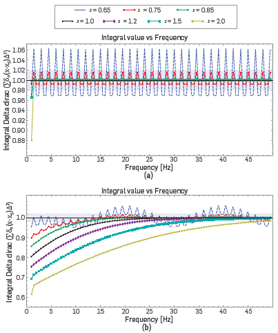
Figure 3 (a) Integral values for discrete Dirac delta calculate for Eq. 9 for different scale factor, assuming the position of the source is x s = 1 Km and z s = 1 Km; (b) Placed at x s = 1 Km and z s = 0.015 Km.
We can see in Figure 3 that the values of l(s,f) remain close to 1 for the scale factor below 1. We can also note that for low frequencies, the integral has a value close to 1 for scale factors s<l, for scaling factors s=[l,2] the integral has values distant to 1. For scale factor s=[0.65,0.75], l(s,f) fluctuates around 1, while for values in the range s=[0.75,1], we see an asymptotic convergence of l(s,f) to 1, for larger values of the frequencies. This behavior is much more desired as in a multlscale approach, this will ensure better performance of the source for larger frequencies.
It can be, therefore, assumed that the correct value for the scale factor, for our tests with sources located in the center of the domain or at the top, should be s=[0.75,1.0].
THE PML
Now, we focus our attention on the properties of the PML and the selection of the parameters m 0 and N xe ,N ze that control its behavior.
We compute the value of the P-wave amplitude of waves propagating in a 2Kmx2Km field. The media has a constant velocity of 2100m/s, Our Ricker source frequency is 30Hz. The constant quality factor is 0=50, using the damping function of Kolsky (see [5]). The solution uses a cell size Δ=λ/G r, where G r = 7, scale factor s=0.75. The position of the source is x 0= 1 Km and z 0 = 1 Km. We conducted several tests on the dispersion and stability of the solution. It was found that for the scales and frequencies of the experiments presented herein, using G r = 7 offers good solutions of the equation in terms of the Low dispersion. In addition, we tested several frequencies, yielding spectra that behave as expected, amplitude values whose highest value is in the main frequency (see [19]).
Figure 4 shows the real, imaginary parts, and modulus of field P-wave with PML (m 0 = f ) and Figure 5 shows the real, imaginary part, and modulus of field P-wave without PML (m 0 = 0) in a medium with constant velocity, attenuation and density for 15 Hz.
The expected result is a symmetrical and spherical field (in agreement with the result shown in Figure 4). However, in Figure 5 the absence of PML presents a perturbation that is not in agreement with the physical setup of the problem. There are some ripples observed in the figure, which are associated to interference of the incident and reflected waves. These waves are reflected at the borders when no PML is acting in the solution. In this figure, we can see the Importance of the PML so that the results are consistent with the physics of the medium we model (an open boundary problem).
In [17], m 0 is chosen based on trial and error; in this work, we propose defining m 0, n xpml and n zpml as a function of frequency. In Figure 6, we show the modulus of field P-wave (mc =3.0) for 3Hz. The figure at the top shows the full field, the figure at the middle shows an horizontal cut at z=1000m, and the figure at the bottom shows an horizontal cut at z=500m. Figure 7 shows the same, with m 0=3.0 for waves of frequency 10Hz.
In this case, we have used the same value of m 0=3.0 at different frequencies. Initially, for frequencies close to 3Hz, It seems that this choice of m0 was adequate; however, after several experiments, it was noticed that the more we increased the frequency, the PML performance started to deteriorate. This is because the term m0 controls the way in which the functions y pml attenuate the amplitude of the wave; the larger the frequency, the faster the attenuating term falls, so m0 must counteract this behavior at high frequencies. Therefore, m0 is frequency dependent.
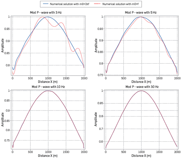
We have noticed for low frequencies that m 0 =f Is not enough to achieve good response. Figure 8 shows a horizontal cut on the modulus of field P-wave at z=100m for a numerical solution using m 0 =f (solid line) and m 0= ω =2πf (dashed line) obtained with the 9-point schemes. For f=3,5,10,30Hz, It is found that the best choice for m 0 is m 0= 2 πf, especially at low frequencies. This choice makes sense considering the way attenuation Is modeled in the PML according to Equations 10 and 11, where we see that the explicit frequency dependence of the damping function Is cancelled.
In addition, n xpml and n zpml are also frequency dependent, which for low frequencies (long wavelengths) should have large values compared to the values of N x and N z such that the amplitude of the pressure field is attenuated correctly. On the other hand, for high frequencies (short wavelengths), only a few points n xpml and n zpml . are needed to damp the pressure field in the region of the PML. After a careful study whereby we systematically varied the frequency and the size of the PML, it was found that a convenient approximation for n xpml and n zpml as a function of frequency is
With c1 = -1.24x10⁻⁶, c2=3.37x10⁻⁴ , c3= -3.07x10⁻² and c4=1.07. We found that using this approximation, the behavior of the PML produces the correct attenuation of the wavefield on the extended domain, in a way that no reflections or spurious information appear in the solution coming from the boundaries. What is most interesting in this approximation is that it provides an automatic way to determine the size of the PML region as a function of the frequency (as one would expect) without the need to find a value through trial and error tests.
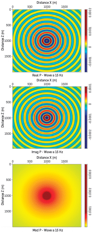
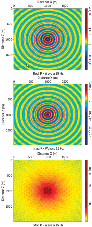
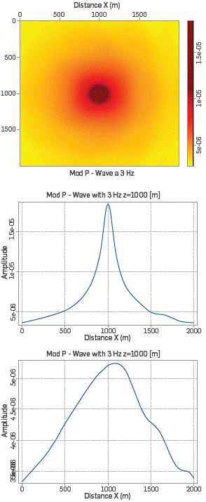
Figure 6 Modulus P-wave with m0=3.0 and f=3Hz. The first figure shows the modulus P-wave for all (x,z) and the following figures show the modulus P-wave for a fixed z.
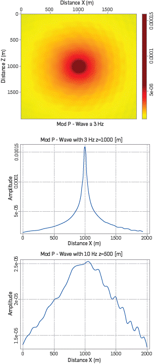
Figure 7 Modulus P-wave with m0=3.0 and f=10Hz. The first figure shows the modulus P-wave for all (x,z) and the following figures show the modulus P-wave for a fixed z.
CONCLUSIONS
In this work, we studied the propagation of waves in a visco-acoustic medium through explicit modeling of the attenuation, using damping functions that allow for dispersion depending on the quality factor. We have implemented a finite difference scheme to solve the problem in frequency domain. Special care was taken regarding the numerical dispersion issues of the modeling, for which we used a mixed grid technique and optimal setup of the intercalated grids to minimize numeric dispersion.
We focused our attention on two particular issues that are loosely discussed in the literature when modeling seismic wave propagation. The first one relates to the discreteness of the source function of the seismic source. The second point we discussed is the selection of the parameters that control the behavior of the PML.
Regarding the source, we show that the condition imposed to fix its behavior is given by the normalization condition of the Dirac delta pulse, and it is considered in the implementation presented in Equation 9, where the behavior of the source term is then controlled through a free parameter s that controls the spread of the source around neighboring cells.
We have shown that parameter s depends non-trivially on the frequency and the position of the source in the field. The dependence on the position of the source is mostly due to the effect of the boundary conditions of the problem; concerning the case of seismic exploration, it should represent a field of air or water boundary in one of the borders. It was found, in particular, that if the source is placed deep down from the border, where the upper boundary effects are neglectable, the parameter s is almost non-dependent on the frequency of the waves. A careful study of the behavior of the model source l(s,f) shows that appropriated values of parameter s that lead to an acceptable normalized behavior of the source term in the range of s=[0.75,1].
When we explored the implementation of the PML, it was noticed that this model ingredient depends on three parameters. The attenuation frequency m 0 , and the scale of the PML zone n_xpml and n zpml . We found that, contrary to what is done in other works (see for example [17]), it is not necessary to test by trial and error the values of m 0 that produce the best results for the performance of the PML. We show that m 0 =2 πf is a very much reasonable choice that also provides the best results out of the PML.
For the size of the PML, after a careful set of tests, a set of relations between n xpml and n zpml and the frequency of the waves was found. This relation facilitates the setup of modeling and inversion experiments intended to achieve optimal process performance.

