1. INTRODUCTION

In the seismic exploration industry, it is necessary to develop techniques to find subsurface characteristics of complex geological areas such as diving wave tomography, Reverse Time migration (RTM), and Full Waveform Inversion (FWI). Full Waveform Inversion Tarantola ^[1] has been recently used to estimate high resolution velocity models of the subsurface. The 2D inversion process involves the modeling of two pressure wavefields, per source used, to obtain the gradient data required to update the velocity model at each iteration. Therefore, due to its high computational cost (in time domain simulation), it is necessary to find strategies to deal with the huge amount of data obtained from the seismic modeling and the execution time involved in the process.

In the last decade, High Performance Computing (HPC) technologies have grown exponentially to handle thousands of millions of mathematical operations per second. In HPC, the most common method used to reduce the execution time is implementing algorithms by using numerous CPU cores and multicore devices such as Graphic Processing Units (GPUs). This is possible due to the parallel programming paradigm. However, in terms of the FWI algorithm, the pressure wavefield volumes represent a large amount of information and memory use. Hence, memory management strategies are useful to minimize this constraint.

The next section describes general aspects of the FWI method used in this work: the wave equation solution and the gradient estimation Plessix ^[2], and our redefinition of the gradient computation based on an inner product property. In section three, there is a description of some state-of-the-art computational strategies available and the usefulness of our proposed way to compute the gradient when using the wavefield reconstruction strategy proposed by Noriega, Ramirez, Abreo and Arce ^[3]. Finally, the experimental environment with its respective analysis are described and the conclusions are shown.

2. THEORETICAL FRAME

Full Waveform Inversion is a non-linear inversion method that iteratively estimates subsurface characteristics such as seismic velocity or density. These parameters are updated until the cost function reaches an adequate value.

Usually, the cost function is defined as

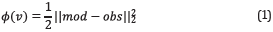
where v ϵ R ^N _x ^xN _z (for the 2D case) is the velocity model, obs is the acquired data and mod is the modeled data. Nx and Nz are the number of elements on the model in the x and z coordinates.

The velocity model can be updated in iteration k+1 using the first two terms of the Taylor series around a previous iteration k velocity model v ^k as

where g(v ^k) represents the gradient of the misfit function, H(v ^k) represents the Hessian matrix, both evaluated at v ^k and α is a scalar factor.

L-BFGS method was defined by Liu and Nocedal ^[4] to calculate an approximation of the product between the inverse of the Hessian matrix and the gradient ([H(v ^k )]^-1 ⋅ g(v ^k)). This approximation uses the last m gradients and velocity models to compute the step forward and requires at least two gradients and two velocity models to obtain the search direction r.

Table 1 shows the pseudocode for this method, where s _k=v _k+1-v _k, y_k=g _k+1-g _k and σ _k=1/y _k ^t s _k. The matrix is approximated by a diagonal with

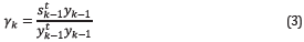
Table 1 L-BFGS Algorithm pseudocode. The search direction r is the product between the inverse of the Hessian matrix and the gradient. 

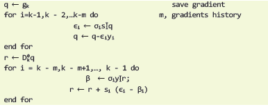
Plessix ^[2] proposed a way to compute the velocity gradient by using the first order adjoint state method, as shown in the mathematical expression below

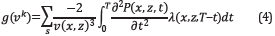
where P is the forward wavefield generated by the source, λ is the backpropagated field of the residual data (the difference between the modeled and acquired data) and s varies according to the number of sources.

The integral operation in the Equation 4 can be written as the inner product between the forward and backpropagated wavefields as

Similarly, for the density information, the gradient can be determined as

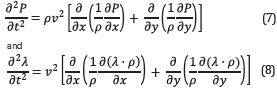
The core of the FWI is the modeling of the wave equation used to obtain the simulated data and the respective adjoint equation and operator used to obtain the inversion gradient. The isotropic acoustic wave equation with variable density is used in this work and the mathematical expressions for the forward modeling and backward modeling are respectively, where ρ is the seismic density. Therefore, a joint inversion with both variables, velocity and density is viable.

The inner product exists as a generalization of the dot product applied to vector spaces and it has the same properties as commutative or multiplication by a scalar factor. Its notation is <.,.>, Additionally, there are different types of linear maps between inner product spaces. The one of interest in this work involves a linear operator as follows:

Being A any linear and symmetric operator and the inner space V, then:

for all x, y ∈ V.

For the second order time derivative wave equation used in this work, the term A is self-adjoint in Equation 9 Bleistein ^[5]. However, when using the first order time derivative velocity-stress formulation, A=∂/(∂t ) and A ^* = - ∂/(∂t).

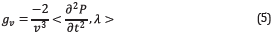
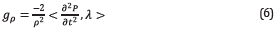
Now, it is possible to redefine the gradient computation as and

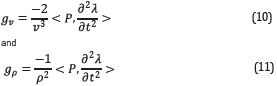
where g _v and g _ρ are the velocity and density gradients, respectively,

HIGH PERFORMANCE COMPUTING IMPLEMENTATION STRATEGIES

The wavefield modeling step, in the FWI, has a computational complexity of 0(N ³) for the 2D case, which represents significant time when increasing the size of the dataset. In terms of RAM consumption, this wavefield volume can use up to hundreds of Gigabytes of memory space. Therefore, there are computational strategies to deal with these problems.

HPC is the field focused on aggregating computing power in a way that the execution performance is much higher than when working with common desktop computers. Therefore, it is possible to reduce the execution time, if so allowed by the algorithm, a couple orders of magnitude van Meel et. Al ^[6].

On the other hand, there are implementation strategies to manage RAM consumption. The Checkpointing strategy showed in Imbert et. al. ^[7] consists on saving a time snapshot (checkpoint) of the wavefield volume each n time steps. Then, the time slides are recomputed between checkpoints, when needed. Thus, the strategy could save up to 90% of memory consumption in the modeling process. Nevertheless, the execution time will increase exponentially making the strategy worthless for big data sizes.

The wavefield reconstruction strategy Noriega, Ramirez, Abreo and Arce ^[3], Yang et. Al. ^[8] (see Figure 1) consists of reconstructing the backward wavefield from the information in the boundaries of the area of interest. It is so that memory consumption can be reduced to less than 5% of the original value but it increases the execution time by a factor of nearly 1.55. The execution time increment is a consequence of an additional forward modeling because the numerical reconstruction of the time derivative of the pressure wavefield becomes unstable.

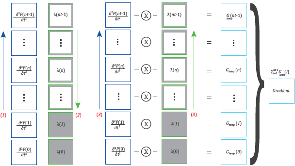
Figure 1 Wavefield reconstruction strategy. First, the forward modeling is performed without saving the pressure wavefield; then, the information at the boundaries of the backward wavefield slides is saved in RAM. Finally, the forward wavefield is recomputed and the backward wavefield is reconstructed while the gradient is calculated. Red numbers are the order in which each modeling is performed. Color arrows indicate the order in which the snapshots of each wavefield are calculated. 

However, the gradient computation proposed in this work (Equations 10 and 11), makes it possible to reconstruct the forward wavefield and apply the time derivative to the backward wavefield as illustrated in Figure 2.

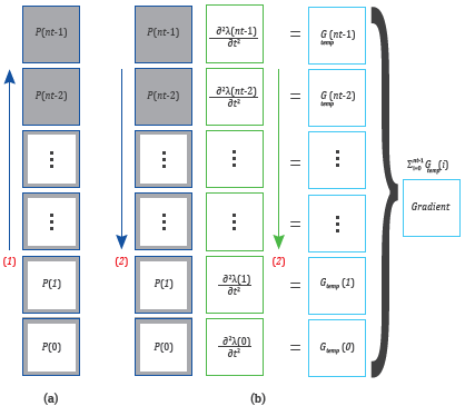
Figure 2 Gradient computation by taking advantage of the inner product property and the wavefield reconstruction strategy. On (a) forward wavefield, boundaries are saved on RAM. On (b) forward wavefield is reconstructed while backward wavefield and gradient are computed. Color arrows indicates the order the snapshots are computed, and red numbers mean the order each modeling is performed. 

3. EXPERIMENT DESCRIPTION

A Canadian overthrust synthetic dataset was created for the CSEG paper by Gray & Marfurt in 1995 (see Figure 3). The model is composed of velocity gradients, faults, a complex topography, and mixed areas of Low and high velocities. The velocity model was widely circulated among Canadian contractor companies in the mid 1990s. As regards density data, it was necessary to use the Lindseth relation Quijada and Stewart ^[9] to generate the original density model. The initial velocity model of the inversion process is a smoothed version of the original model (see Figure 4).

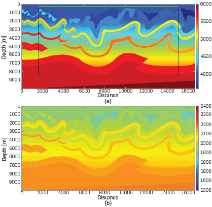
Figure 3 Canadian Foothills velocity model. (a) Original velocity model. The area outside the black lines represents the CPML zone. The top gray line represents the position of the receivers for each source used in all the experiments (each pixel is a receiver). The magenta dots represent the position for all the sources used in all the experiments. (b) Original density model used in combination with the original velocity model to generate the observed data. 

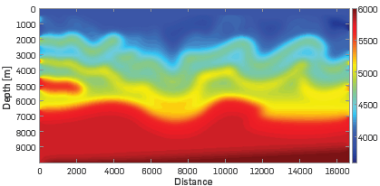
Figure 4 Initial velocity model for the multiscale process. The matrix was obtained by applying an average filter 150 times over the original velocity model. 

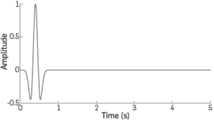
The ricker wavelet (see Figure 5) was used to generate both, the observed data and the modeled data at each FWI iteration. The mathematical expression used to obtain the source is

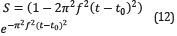
where f is the central frequency, t is the time window and t₀ is a time delay. Sources were shoted from a flat surface corresponding to the upper limit of the model.

Figure 5 Ricker wavelet with a central frequency of 3 [Hz]. 

A multiscale frequency approach was used to obtain better results Mao et. al. ^[10]. The frequency sweep process consists on start by using a low central frequency wavelet (f =3[Hz] for our experiments) to model the pressure wavefield, run the FWI and obtain a velocity model. Then this final model is used as the initial guess for a new inversion process where the central frequency is higher and so on until covering the desired frequency bandwidth.

As regards implementation, the Finite Difference in Time Domain method (FDTD) is used to discretize the wave equation. The time and spatial discretization is second order and eight order stencil, respectively, using the staggered grid method. Then, the mathematical expressions 7 and 8 can be expressed as

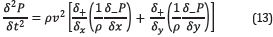
And

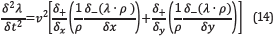
respectively, being

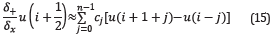
And

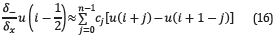
where c _j are the first derivative coefficients of the FDTD stencil.

CUDA C programming Language is used to take advantage of the computational power of GPUs, by implementing the wavefield modeling with the parallel programming paradigm. Each time snapshot is computed on the GPU, reducing the execution time in comparison to a serial implementation.

The Convolutional Perfectly Matched Layer (CPML) Pasalic et, al. ^[11] is a well-known boundary condition used to simulate the extension of the FDTD lattice to infinity and it is used as the non-natural boundary in our implementation (see Figure 3).

In terms of RAM consumption, the equation to calculate the amount of memory used (in Mebibytes where 1 Mebibyte=2²⁰ bytes. Megabyte =10⁶ bytes) by this implementation, when there is no reconstruction strategy, is given by expression 17,

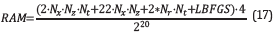
where N _x -N _z -N _t is the size of each, forward and backward wavefield Additionally, there are other variables, with the same size of the velocity and density models, necessary to compute the pressure wavefields, the information related to boundary conditions, etc. The N _r-N _t term is the space used by each, the modeled and observed data per source used in the process, where N _r is the number of receivers and the term LBFGS is the memory used by the variables associated to the L-BFGS method with a value of 43x2¹⁷ for this work.

The pressure wavefields P and λ are the most expensive variables and that is why the reconstruction strategy is necessary when the model dimensions increase and the available RAM on the GPU is not enough to hold all the data

Expression 18 is used to compute the RAM consumption when the reconstruction strategy is applied to the implementation

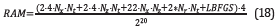
where the term 4⋅N _x⋅N _t is the space used by the information saved from each, the top and bottom boundaries of the area of interest each time slide of the pressure wavefield, and 4⋅N _x⋅N _t is the space used by the information saved from each, the left and right boundaries of the area of interest for each time slide of the pressure wavefield.

If the model dimensions increase so that the RAM consumption exceeds the GPU capacity (e.g. when the implementation is used to process real seismic data volumes) the same expression can be applied to the total system memory (GPU RAM and the memory accessed by the CPU) where it is necessary to add the penalties of transferring data from GPU RAM to CPU RAM and vice versa

The cluster used to run the experiments consists of 3 nodes with two Intel Xeon E-2620 v3 CPU, two Nvidia Tesla K40 GPU and 256 GB of ECC RAM per node. The Nvidia Cuda Compiler driver version 6.5 is used. The GNU Compiler Collection version used is 4.8.4 on Linux 3.16 - Debian Jessie.

The implementation process is focused on distributing the number of gradients per iteration (directly related to the number of sources used in the process) over all the computing nodes and improving performance, in terms of RAM consumption, per node. Thus, if more computing hardware is added to the system, the speedup factor would increase (more computing nodes will process more source wavefields at a time)

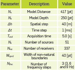
Other important parameters of the experiments are shown in Table 2.

Table 2 Main parameters of FWI used to run the experiments. 

4. RESULTS

Thirty-five iterations were carried out per frequency step. Figures 6, 7 and 8 show the final velocity model for f=3[Hz], f=6[Hz] and f=9[Hz], respectively.

Figure 6 Final velocity model of each experiment with a central frequency of 3 [Hz]. 

Figure 7 Final velocity model of each experiment with a central frequency of 6 [Hz]. 

Figure 8 Final velocity model of each experiment with a central frequency of 9 [Hz]. 

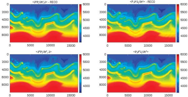
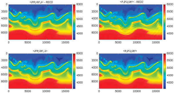
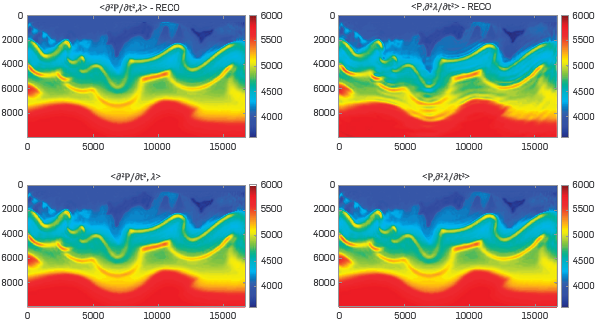
The experiment comparison is focused on whether the wavefield reconstruction strategy is or is not used and whether the traditional way to compute the gradient or our approach is implemented. The RECO word means that the wavefield reconstruction strategy was used. The term inside the "<>" means whether the traditional way to compute the gradient is used or not.

It is to be noted that, with a central frequency of 9 [Hz], the changes over the velocity model are minimal as compared with the previous frequency value and an additional frequency step may not be necessary. Therefore, to obtain a mathematical measure of the results, the Peak Signal to Noise Ratio was calculated for each experiment. Figures 9, 10, and 11 show the PSNR at each FWI Iteration for all the experiments. The density data was updated with Its respective gradient (Equation 11) through the inversion process, and the initial density model was obtained through the same process of the initial velocity model.

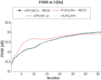
Figure 9 Peak Signal to Noise Ratio between the velocity model at each FWI iteration and the original velocity model with a ricker central frequency of 3 [Hz]. 

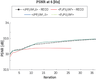
Figure 10 Peak Signal to Noise Ratio between the velocity model at each FWI iteration and the original velocity model with a ricker central frequency of 6 [Hz], Note that the experiment that combines the wavefield reconstruction and the gradient computation proposed in this work just reached 26 iterations. 

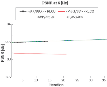
Figure 11 PSNR between the velocity model at each FWI iteration and the original velocity model with a ricker central frequency of 9 [Hz]. At this stage, the experiments that used the wavefield reconstruction strategy did not complete all the 35 iterations. The process stopped because the algorithm did not find any better model to still decreasing the cost function at these iterations. 

It should be noted that, when using the wavefield reconstruction strategy, the numerical error associated with the reconstruction step decreases the quality of the result and some of the experiments did not reach all the 35 iterations but the difference in dB of the PSNR curve values are below 0.5.

There is also a measurement of the time consumed by the inversion process (Table 3) when using a single GPU and when using the whole computing system (to analyze the effect of using MPI for the inter-node communication).

Table 3 Execution time for different versions of the implementation. The word RECO means that the reconstruction strategy was applied and the terms inside the angle brackets mean whether the traditional way to compute the gradient or the re-definition of the gradient computation was used. Note that, the re-definition of the gradient computation by applying the inner product property reduces the time penalty of the reconstruction strategy. 

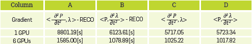
Note that, as ^[3] shows, the implementation with the reconstruction strategy and the traditional way to compute the gradient (column A) Is affected by a time penalty of 55%, approximately, in comparison with the implementations that do not use the reconstruction strategy (columns C and D). However, when combining this reconstruction strategy and the re-definition of the gradient by applying the inner product property (column B), the time penalty Is just near 10% as compared with the results in columns C and D. The slightly differences in the execution time between columns C and D are associated to the effect of other resource utilization in the computing system, but these differences are minimal and can be ignored.

Additionally, it seems that the time penalty associated to data transfer between computing nodes is acceptable. The obtained speed up working with six GPUs (three computing nodes), instead of a single GPU, is approximately 5.6x over an expected speed up of 6x (if data transfer time between compute nodes and other devices Is zero) for all the versions of the implementation

Table 4 RAM used by different versions of the implementation. The word RECO means that the reconstruction strategy was applied and the terms inside the angle brackets mean whether the traditional way to compute the gradient or the re-definition of the gradient computation was used. Second row is the values obtained when applying equations 17 (without reconstruction strategy) and 18 (reconstruction strategy) to calculate the used memory. Third row is the measurement given by the nvidia-smi command of how much memory of the specific GPU is on use. 

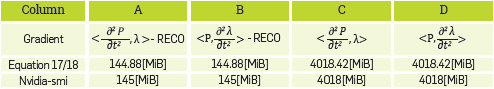
It is to be noted that, the pair of implementations that use the reconstruction strategy (columns A and B) and the pair that do not use it (columns C and D) have the same memory usage measurements due to the allocated space on RAM is the same, but the applied operations are different.

CONCLUSIONS

This work proposes a different expression to compute the FWI gradient by using an inner product property.

The behaviour of the experiments when using the traditional way to compute the gradient and the expression proposed in this work, without applying the wavefield reconstruction strategy, are identical.

It is possible that the error associated with the reconstruction strategy could introduce values to the velocity models that benefits the behaviour of the PSNR curve at the beginning of the process.

However, through the multiscale stages, this error will be higher and the impact on the result will be negative as can be observed in Figure 11.

The experiments with the wavefield reconstruction strategy implementation show a different behaviour in comparison with other tests (less FWI iterations as seen in Figures 10 and 11 and final velocity models with some artifacts). However, the magnitudes in the PSNR curves show differences below 0.5 [dB] and the strategy is still considered useful to increase the performance of the inversion method.

The experiments showed that, when using the reconstruction strategy, at the end of the multiscale process, the numerical error introduced by the time derivative of the backward wavefield (the interaction of multiple sources) is higher than the numerical error introduced by the reconstruction technique.

If the model dimensions require the use of the reconstruction strategy for the inversion problem, the combination of the strategy with the gradient expression proposed in this work will increase the FWI performance in terms of RAM consumption without compromising the execution time.

The numerical error presented in this paper could increase as a result of adding noise to the source and the adjoint wavefield; therefore, it is necessary to evaluate the effect of noise over the reconstruction strategy as further work. Additionally, for real data volumes, it is necessary to analyze the sources and receiver's distribution along the acquisition to obtain the ratio, if it exists, between the numerical error of the reconstruction strategy as a consequence of erroneous positions.

It is necessary to analyze the effect of executing the implementation on a larger computing system (e.g. dozens or hundreds of computing nodes) in terms of speed up and other resources' utilization. Additionally, it is expected that this implementation will be useful to process larger dimension seismic data, given the reduced RAM consumption and execution time.