1. INTRODUCTION
Recently, full waveform inversion (FWI) has become an attractive technique for the estimation of high resolution parameters of the Earth's subsurface. FWI is formulated as a local optimization problem, where first-order or pre-conditioned first-order functions of the misfit between observed and modeled data, are used to find the search direction to the nearest minimum [1], [2] The inverse of the Hessian matrix not only guides the descent direction in the local optimization method, but also allows quantifying the uncertainty of the parameters estimated with FWI. For uncertainty quantification, the inverse of the Hessian matrix is related to the covariance matrix of the estimated set of parameters when Bayesian inference and Gaussian models are used to model the error between the real and estimated parameters [3] In fact, uncertainty of the FWI can be quantified using Gaussian model assumptions when 𝓵2 error norms are used as data-fitting term[4]. The second-order information of the misfit function, known as the Hessian matrix, is usually neglected in FWI implementations because computing this matrix for large scale problems (real inverse problems) is computationally unfeasible. Several methods have been proposed to compute approximations of the Hessian matrices, such as the BFGS and its variants [5], Newton, Gauss-Newton and Levenberg-Marquardt [6].
The main contributions of this work are two-fold. First, we provide the formulation of the adjoint wavefields used to compute the Hessian matrix using the Second Order Adjoint State Method (SOASM) for the acoustic and isotropic case. Special emphasis is placed on computing the adjoint wavefields using parallel programming such that a feasible implementation on GPUs is proposed. Second, we provide the link between the Hessian matrix and the uncertainty quantification of the estimated velocity model obtained with the acoustic and isotropic FWI. This is a function of the uncertainty of an a priori velocity model. The analysis of uncertainty of the estimated parameters are performed for different central frequencies of the source. Thus, we can identify which parameters are better resolved at different frequencies.
The exact Hessian matrix is obtained via the SOASM, which computes Hessian matrix-vector products by using auxiliary variables called adjoint variables [6]- [10]. As regards the acoustic and isotropic case, we obtained every column of the Hessian matrix using four wave propagations via finite-differences in time-domain (FDTD). In the FDTD scheme, every spatial point of a pressure wavefield snapshot can be computed independently, which generates an intrinsic parallelism in the numerical computation of the wave propagations. In this work, we exploit the high level of parallelism of the pressure wavefield modelled with FDTD through the use of parallel architectures as GPUs [11], for reducing the computational cost of the Hessian matrix computation.
This paper is organized as follows: the second section presents the adjoint wavefield equations and the pseudo-code of the parallel implementation on a GPU architecture. The third section describes the strategy for quantifying uncertainty of the estimated parameters after FWI. The fourth and fifth sections show the experiment conducted to test the SOASM implementation and the corresponding results with synthetic velocity models, respectively.
2. THEORETICAL FRAME
In this section, we describe the adjoint wavefields that are used to obtain Hessian-vector products. In particular, we formulate the adjoint wavefields for the acoustic and constant density model of a seismic source wave propagation. Furthermore, the pseudocode of the adjoint wavefields implementation is presented and its computational cost on CPUs and GPUs is also discussed.
Let H(v) be the Hessian matrix as a function of a given velocity model v. The l
th column of H(v) can be obtained through the interaction of the wavefields u and α with the adjoint wavefields  and
and  as
as
where w i is the vector used to select the column of the Hessian matrix and <a,b> is the inner product operator between vectors a and b . The sources of the forward wavefields are f and Φw, and N xxN z represents the model size.
COMPUTING THE DERIVATIVE OF THE WAVEFIELD u
The wavefield u produced by a seismic source that propagates through an acoustic and isotropic medium can be modeled in two-dimensions for constant density as
where v(x,z) is the acoustic velocity of the medium as a function of the spatial variables x and z; u denotes the scalar pressure field, t is the time variable, and f(x,z) represents the seismic source. The wavefield u can be numerically obtained by using a finite-difference stencil in time domain (FDTD), with the initial conditions given by u(x,z,0) = 0, ∂u/∂t(x,z,0) = 0. The non-natural boundaries (left, right and bottom sides) of the FDTD numerical implementation are handled using Convolutional Perfectly Matched Layer (CPML), proposed by [12].
Equation 2 can be re-written in a general form as
where L represents the acoustic wave equation. The derivative of Equation 3 with respect to the model parameters is given by
Once the auxiliary field ∂ 2 u/∂t 2 has been computed, the solution for Equation 4 is easily obtained by multiplying the auxiliary field by the scale factor -2/v 3 (x,z). This is shown in steps 1 and 2 of Algorithm 1.
COMPUTING THE ADJOINT WAVEFIELD 
Let the adjoint wavefield  , in operator form, be given by
where f† is defined in Equation 7. The derivative of previous operator with respect to the model parameters v is then
As the acoustic and isotropic wave equation (Equation 2) is used for computing the forward wavefield u, its adjoint wavefield can be computed using the same wave equation, because the system is self-adjoint. However, the propagation direction changes and the adjoint wavefield  represents a back-propagation, meaning that the final conditions of the problem are defined as
  (x,z,T)=0 and (∂
 /∂t(x,z,T) = 0, for a final time T.
In order to compute the adjoint wavefield  , the receivers become sources (adjoint source) and the real source disappears as a consequence of the least square minimization of the cost function. The mathematical expression for the new set of sources is given by
where dobs represents the measured pressure wavefield at the surface level (seismic traces), dmod are the modeled seismic traces and, R†(⋅) represents the operator to flip the vector of residuals. Note that the residuals, used as sources, are injected from the final sample to the first sample. This is shown in steps 3 and 4 of Algorithm 1.
COMPUTING THE DERIVATIVE OF α
Before obtaining ∂(L(α,v)-Φw)/∂v, the auxiliar source Φw, and the wavefield α should be defined. Let Φw be an auxiliary source, defined by
where Nx is the number of grid points in the x direction, Nz is the number of points in the z direction, and wi (j) is a perturbation vector having zero-value in all but the jth coordinate. A non-zero value determines the location for the perturbation, which corresponds to one column vector of the Hessian matrix. If more than one perturbation is selected (i.e., more than one element in the vector wi (j) is different from zero) then the Hessian-vector-products compute a column that represents a linear combination of the selected Hessian matrix columns. The auxiliary wavefield α is a forward wavefield computed when the source is Φw, and the initial conditions are α(x,z,0)=0 and ∂α(x,z,0)/∂t=0.
The derivative of the wavefield α with respect to the model parameters v, is given by
Equation 9 represents the interaction between the forward field α and the perturbation of the geophysical model. This is shown in steps 5, 6 and 7 of Algorithm 1.
COMPUTING THE ADJOINT WAVEFIELD 
The adjoint wavefield  is computed using as source
where Rα is the pressure field at the surface, obtained with the auxiliary field α. This means that the adjoint wavefield  uses the number of receivers and the perturbations of the geophysical model as sources. Also, the final conditions are
  (x,z,T)=0 and ((∂
 )/∂t) (x,z,T)=0. Note that (∂2
 )/∂t2) was obtained previously.
The computation of the adjoint wavefield  is shown in step 8 of Algorithm 1.
COMPUTING THE SECOND DERIVATE OF THE WAVEFIELD u
The second derivative of the forward wavefield u for the acoustic and isotropic case is given by
This is shown in step 9 of Algorithm 1.
Finally, as the terms in Equation 1 are known and the columns of the Hessian matrix can be obtained. A physical interpretation of each kernel in Equation 1 was presented by Fichtner [10].
IMPLEMENTATION OF THE SOASM ON GPUS
The computational complexity of the wave propagation modeling is in the order of (N 3) for a squared synthetic model with N 2 elements and N time steps. However, if the same task is performed on a GPU then the execution time is reduced, as if the number of operations were (N), due to the parallelism level at each time step [11].
Now, according to the SOASM algorithm, the modeling of four wavefields(u,α, and
and  ) is needed to compute one column of the Hessian matrix. Furthermore, as a model of N2 elements produces a Hessian matrix of N2 columns, then the full Hessian matrix has a computational cost of (4N5) for the SOASM. Nonetheless, when the SOASM is implemented on a GPU, the execution time is reduced as if the number of operations were (4N3). The reduction of two orders of magnitude in the execution time of the full Hessian matrix makes it feasible for uncertainty quantification.
UNCERTAINTY QUANTIFICATION
This section describes the link between the posterior covariance and the Hessian matrix using Bayesian inference. The posterior probability function of the model v given the observations dobs can be expressed as
where ρ(v) is the a priori density function of the model parameters and ρ(v|dobs) is the likelihood function that relates the observations with the given model parameters. If the likelihood and the a priori functions follow Gaussian multivariate distributions, and the relation between the observations and the model parameters is linear, then the posterior probability function ρ(v|dobs) is also Gaussian [3], and it is given by
where  is the maximum likelihood solution of the model parameters and Σ
post is the posterior covariance. The posterior covariance matrix can be obtained as a function of the Hessian matrix of the cost function H, and the a priori covariance matrix Σ
prior, as follows
The a priori covariance matrix is chosen such that the correlations between model parameters are included. Assuming that the model parameters are uncorrelated and identically distributed, the a priori covariance matrix is given by
where I is the identity matrix, and the elements of the diagonal are the variance σ2
prior. Even though this is not a realistic model for the prior correlation of the model parameters, because usually parameters located at neighboring positions belong to the same class, the computation of the inverse  prior is simple. Despite the assumption of uncorrelated model parameters in the prior density function of the model parameters, it is possible that the posterior covariance matrix has elements off-diagonal that are nonzero. The posterior correlation between the parameters
  and
and  means that they were not independently resolved by the observed data during the full waveform inversion.
3. EXPERIMENTAL DEVELOPMENT
In this section, we describe the experiment that has been formulated to evaluate the Hessian matrix computation for the uncertainty quantification of the velocity model obtained after multi-scale FWI. We also evaluate the computational performance of obtaining the Hessian matrix via SOASM using GPUs.
EXPERIMENT DESCRIPTION
The synthetic true velocity model used to obtain the observed data d obs is depicted in Figure 1. The velocity model is of size N xxN z=211x68, with a spatial grid of 25 m (Δx=Δz=25 m). The background velocity is 2000 m/s and the diffracting squared area has a velocity of 2500 m/s. The diffracting element is a square of size 9x9 centered at the position x = 2650 m and z = 850 m. The observed and modeled data were produced using a set of 171 receivers placed in line at a depth of 125 m every 25 m, starting from the position 525 m to the position 4775 m. Each receiver recorded 3.5 s at a time step of 4 ms (Δt=4e -3s).
Different number of sources were Located at z=125 m and all of them have the source wavelet defined by
where f 0 Hz is the central frequency, and t 0 is a time delay parameter All the parameters of the numerical implementation were set to satisfy the Courant's stability criterion with a CPML area=20 (grid points). Please refer to [12] for the definition of the variables used in the CPML.
The velocity model used as starting point for a multi-scale FWI approach [13] is the same as Figure 1 but without the diffracting square (white square), where the central frequencies of the source wavelet were set to 3 Hz, 6 Hz and 9 Hz. The implementation uses a second and eighth order stencil of FDTD for approximating the time and spatial derivatives, respectively. We compute the gradient through the inner product between the derivative of the forward modeling and the residuals back propagation as it is proposed by Plessix [14] in Equation 36. Besides, the gradient computation uses CUDA-C for GPUs [15]- [16], For the first FWI iteration, we used linear interpolation to compute the step forward, and for the subsequent 39 Iterations, we used L-BFGS [17]. The resulting velocity model of the first inversion (f 0=3Hz) becomes the starting model for the second inversion (f 0=6 Hz). This process is repeated for the last frequency (f 0=9 Hz). The sources were placed at a depth of S z=125 m and their spatial location were obtained using the following equation
where a is the grid position of the first source (a=21), b the grid position of the last source (b=191), n the number of sources (n=1,51), S R the spatial resolution (S R=25 m) and ⌊ ⌉ represents the nearest integer operator.
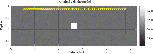
Figure 1 Original velocity model [m/s] used in FWI with a background velocity of 2000 m/s and a diffracting square of 2500 m/s. The initial velocity model only has the background velocity of 2000 m/s and in both cases, the area out of the red square represents the CPML zone (left, right and down) and the free surface conditions (up). The source positions are marked in yellow and the 171 receivers are placed from the position 525 m to the position 4775 m all of them at the same depth of the sources (125 m).
The estimated velocities for the multi-scale process for one and fifty-one sources are depicted in Figure 2a and Figure 2b, respectively. In Figure 2 can be noticed that the estimated velocity for the diffracting square is closer to the true velocity as the number of sources increases. In fact, the FWI method is able to estimate the velocities inside the diffracting area with at least 51 sources. However, the zone below the diffracting area cannot be updated correctly during the inversion due to the acquisition geometry.
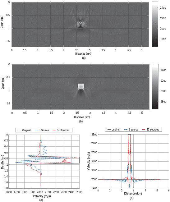
Figure 2 Multi-scale FWI results using the central frequencies f0=3, 6 and 9 Hz with 40 iterations per frequency step. Results for (a) 1 source and (b) 51 sources with the vertical log (c) taken at x=2.65 Km and the horizontal log (d) placed at z=0.85 Km of depth.
The Hessian matrix associated to the velocity model estimated with the FWI multi-scale approach for one source is shown in Figure 3, Note that the Hessian matrix, obtained via SOASM, differs from the one given by Virieux (see Figure 2a in [1]) because it is not symmetric. The lack of symmetry is a consequence of using superficial sources and receivers only. To obtain a symmetric Hessian matrix, an array of sources and receivers should be located enclosing the area of interest [1], but this is not feasible in real seismic acquisitions. Also, the resulting Hessian matrix is not positive definite, which can be explained by the fact that in a surface acquisition, we do not have sufficient observations to build a high-dimensional Hessian (or covariance) matrix from a reduced number of measurements. This can also be evidenced through the magnitude of the eigenvalues of the Hessian matrix, which rapidly decay to zero (see Figure 4).
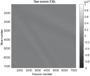
Figure 3 Hessian matrix for the velocity model estimated with multi-scale FWI using 1 source and 171 receivers (see Figure 2a). This Hessian matrix describes the interaction of the 7182 elements inside the red square (see Figure 1).
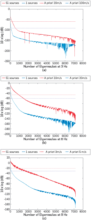
Figure 4 Eigenvalues of the Hessian Matrices computed at (a) 3 Hz, (b) 6~Hz and (c) 9~Hz for one source and fifty-one sources. These eigenvalues describe the interaction of the 7182 elements inside the red square (see Figure 1).
UNCERTAINTY QUANTIFICATION
The posterior covariance matrix can be obtained using Equation 14 for the estimated velocity models with a multi scale FWI method The Hessian matrix H is obtained via SOASM and the a priori covariance is obtained assuming uncorrelated pixels, as expressed in Equation 15.
For the estimated models using 1 and 51 sources, shown in Figure 2, the uncertainty of the model can be quantified using three different Hessian matrices, each associated to a central wavelet frequency (3, 6 and 9 Hz). The posterior covariance matrices Σ post are obtained by setting the a priori standard deviation for all pixels in σa=3, 5, 10, 20 and, 100 m/s. Figure 5 and Figure 6 depict the standard deviation of each pixel in the model, for one and fifty-one sources, which correspond to the square diagonal elements of the posterior covariance matrix Σ post. Note in Figure 5 and Figure 6 that the posterior variance decreases in comparison to the prior variance, in the area that is properly illuminated by the sources. For only one source, the illumination angle is smaller than for 51 sources, and thus only a small portion of the model is properly updated during the inversion process. Also, note that for the smaller frequency (3 Hz), the uncertainty can only be quantified coarsely, whereas for the larger frequency (9 Hz), the uncertainty can be quantified at a Level of pixel.
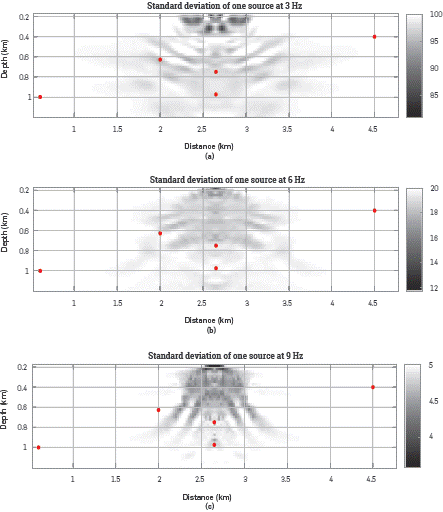
Figure 5 Posterior standard deviations, computed using Equation (14) at (a) 3 Hz, (b) 6 Hz and, (c) 9 Hz, for the velocity model estimated with 1 source (see Figure 2a). The Hessian matrices are computed using the SOASM and the a priori covariances are obtained using Equation 15 with the a priori standard deviations: (a) 100 m/s, (b) 20 m/s and, (c) 5 m/s. The red dots are placed at five points with different illumination.
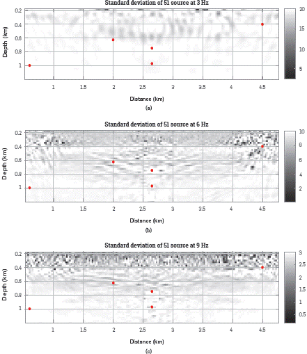
Figure 6 Posterior standard deviations, computed using Equation 14 at (a) 3 Hz, (b) 6 Hz and, (c) 9 Hz, for the velocity model estimated with 51 sources (see Figure 2b). The Hessian matrices are computed using the SOASM and the a priori covariances are obtained using Equation 15 with the a priori standard deviations: (a) 20 m/s, (b) 10 m/s and, (c) 3 m/s. The red dots are placed at five points with different illumination.
In addition, the uncertainty of the prior velocity model is reduced due to the "new" information brought by the observations in the inversion process. The comparison between posterior uncertainties and prior uncertainties can also be quantified. The uncertainty reduction of the i th pixel in the model, after the multi-scale FWI is measured as
where  is the posterior variance of the i
th pixel in the model. A value of VR
i
=0 or negative means that no-new information was brought from the observed data on the i
th pixel. A positive value of VRi means that the inversion method added new information on the i
th pixel and thus the uncertainty of the posterior variance
  is smaller than the a priori variance.
Information that complements the FWI results. The Hessian matrix is mainly affected by the ¡ L Lu mi nation area produced by sources and receivers, the source Figure 7 and Figure 8 illustrate the variance reduction. The uncertainty reduction given in Figure 7a shows that only a few parameters in the model have been "correctly" resolved, This occurs since the posterior covariance is obtained using a low frequency wavelet as source, which quantifies the uncertainty of a group of neighboring pixels instead of the uncertainty of one single pixel at the time. Figure 7b and Figure 7c show the uncertainty reduction using sources with higher frequencies. Particularly, Figure 7c shows the reduction in the uncertainty for every single parameter n the model, and a higher reduction is obtained (as expected) in the area underneath the source.
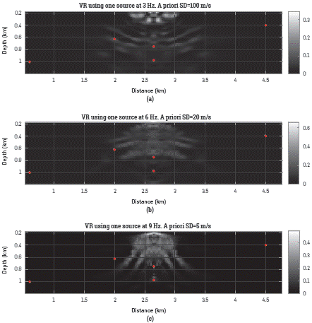
Figure 7 Variance reduction computed with Equation 18 for the posterior standard deviations illustrates in Figure 5. For these results the a priori variances were set to (a) 10000 [m/s]2 for 3 Hz, (b) 400 [m/s]2 for 6 Hz and (c) 25 [m/s]2 for 9 Hz. The red dots are placed at five points with different illumination.
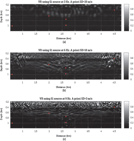
Figure 8 Variance reduction computed with Equation 18 for the posterior standard deviations illustrates in Figure 6. For these results the a priori variances were set to (a) 400 [m/s]2 for 3 Hz, (b) 100 [m/s]2 for 6 Hz and (c) 9 [m/s]2 for 9 Hz. The red dots are placed at five points with different illumination.
The a priori standard deviations were selected to define the lowest eigenvalues of the Hessian matrices accepted to compute the posterior covariance matrices. As the eigenvalues behavior vary when both the number of sources and the source frequency change then each experiment uses its own a priori standard deviation (see Figure 4). If the a priori standard deviation is set to a very small value then the information provided by the Hessian matrix is almost neglected for the posterior covariance. On the other hand, a large a priori standard deviation value produces a posterior covariance matrix that can be affected by the small eigenvalues of the Hessian matrix generating undesired effects (e.g. complex: negative or extremely high variance values). For the six tests, the a priori variances were selected to obtain as much information as possible from the Hessian matrices avoiding the undesired effects of the small eigenvalues.
Five pixels in the velocity model were selected to identify areas with Low illumination (P 1=(0.6,1) km and P 2=(4.5,0.4) km), with high illumination and under a high velocity contrast area (P 3=(2.65,0.975) km) and with high illumination over a high velocity area (P 4=(2,0.625) km and P 5=(2.65,0.75) km). The true velocity value for P 1, P 2, P 3 and P 4 is 2000 m/s (outside the diffracting square) and for P 5 is 2500 m/s (inside the diffracting square). The pixels are marked in red color in Figure 5, Figure 6, Figure 7, and Figure 8. For all the tests P 1, P 2 and P 3 were never updated as a consequence of the lack of illumination or the interference produced by the diffracting square. The standard deviation for P 4 and P 5 are affected by the source frequency, the number of sources and σPrior as Figure 5 and Figure 6 illustrates.
COMPUTATIONAL PERFORMANCE
The cost of computing the full Hessian matrix using FDTD, in terms of execution time and memory resources, is high since four wavefield propagations need to be obtained for each column. In particular we evaluate the performance of computing a single column when the FDTD approximation uses a second order stencil for time derivative and an eighth order stencil for the spatial derivatives. Two implementations are evaluated: (1) A serial ANSI-C implementation on an Intel(R) Xeon(R) E5-2609 and (2) a CUDA-C implementation on a Nvidia(R) GPU K40c. The execution times of one single column of the Hessian matrix are presented in Table 1. Besides, Table 2 summarizes the execution times and RAM requirements by the CUDA-C implementation to compute the full Hessian matrix. Note in Table 2 that increasing the number of sources does not increase the RAM required, but instead the computational cost increases linearly with the number of sources. The execution times of the full Hessian matrix for the serial ANSI-C implementation are not presented in Table 2, as these are not computationally feasible.
Table 2 Execution times required for computing one-column of the Hessian matrix in CPU (Intel(R) Xeon(R) E5-2609) and GPU (Tesla K40c).

4. RESULTS ANALYSIS
The Hessian matrix provides valuable information for resolution uncertainty analysis and radiation patterns identification [18] Therefore, computational strategies are needed to make feasible the use of the Hessian matrix. In this work, it has been demonstrated that GPU architectures make feasible the implementation of the second-order adjoint method because the execution time is reduced in two orders of magnitude.
This work presents a parallel implementation of the Hessian matrix-vector products using GPU architectures. The implementation uses the FDTD approximation to compute the wavefield propagations required by the SOASM.
We presented a practical method to compute the standard deviation over the final results (σp) from the a priori variance  and HSOASM. Also, a variance reduction (VR) is computed to define the areas with less uncertainty. It is shown that VR growths when the source frequency and the number of sources increase. However a statistical analysis fails for P1 P2 and P3 because they are not correctly illuminated.
According to Table 2, the computational cost of obtaining the Hessian matrix has a linear behavior when the number of sources change. However, the main concern about computing the Hessian matrix arises when the model size increases given that the computational cost for the 2D implementation is (4N 5). To overcome this problem a cluster of GPUs that divides the load over all the nodes can be used. Also, the computation of the Hessian matrix only for the area of interest decreases the computational cost.
The eigenvalues of a matrix are useful to identify, classify and compare set of matrices through characteristics as the condition number, the rank and the trace [19]. In the theoretical case, if the velocity model has been correctly resolved then the rank of the Hessian matrix evaluated at that point equals the number of model dimensions (i.e., N xxN z) and the condition number equals one because all the eigenvalues have a magnitude close to one.
In this case, the theoretical behavior of the Hessian matrix near the solution is used as a reference to define whether the velocity models are improving after the FWI. Figure 4 illustrates the eigenvalue magnitudes of the Hessian matrices computed from the FWI results at 3 Hz, 6 Hz and 9 Hz for one and fifty-one sources including the 7011 dimensions (171x41). The eigenvalues of all the Hessian matrices are non-zero and their magnitudes are above -250 dB. This produces full rank matrices (i.e., rank=N x×N z=7182) for all the cases. Besides, if the number of sources increases from one to fifty-one then the eigenvalue magnitudes also increase. But, in all cases the results are still far from the theoretical behavior of the Hessian matrix because the condition numbers are much greater than one due to the ratio of the largest singular value to the smallest singular value is also much greater than one.
CONCLUSIONS
Hessian matrices are key for decision-making processes, as they provide new frequency used for the Hessian kernels computation the resolution of the estimated velocity model and the numerical error of the implementation. Therefore, a deepest sensitivity analysis must be done on how the above parameters affect the Hessian matrix. Finally, our implementation makes it feasible to obtain the Hessian matrix for small models. Nonetheless, other computational strategies must be explored to reduce both RAM requirements and execution time, before the SOASM can be successfully applied on real data.


