1. INTRODUCTION

Reverse time migration (RTM) is an imaging technique that was introduced independently by several works around the 1980's ^[1]-[4], but has been extensively used only in the last two decades because of the computational resources needed to implement it. Despite its high computational cost, RTM is nowadays the algorithm of choice to produce seismic images in complex areas because it can be used in zones with strong variations in the velocity of propagation, and can map subsurface structures with any dip to create good images of zones of interest like those under and around salt domes where hydrocarbon reservoirs can be found. The classical RTM algorithm produces images of the earth's subsurface by modelling the source wave field and back propagation of registered data at surface as seismograms. This procedure uses the wave equation (acoustic or elastic) where each seismogram's trace (inverted in time) enters as the source term. When this propagation procedure registers all seismic traces simultaneously, it produces what is known as back-propagated wave field P _b (x,y,z,t), where x, y and z are the spatial coordinates and t is time. This field carries information about the interfaces that produced the reflections. To create the RTM image, the simulation of the seismic source propagation is also necessary. The functional form of the artificial seismic pulse is modeled mathematically and introduced as the source term in the same wave equation used for the back propagation. The result is the forward propagated field, P _f (x,y,z,t). P _f and P _b should coincide in space and time on the sub surface regions where the field was reflected.

Before the use of RTM algorithms was popular, the most common techniques used to produce seismic images were based on field extrapolation in the Fourier domain. This method is known as One-Way Wave Equation, OWWE, or wave field extrapolation as it takes the field that was registered in the surface by the seismic geophones and extrapolates it back into the Earth's interior to predict the location of the reflecting structures or strata where they came from ^[5]-^[7]. This method is much faster and requires less memory, but has some drawbacks: it cannot handle media with strong horizontal variation in wave velocity and also fails to produce good images in the regions of the Earth's subsurface where the strata have large dips ^[7]. These zones can be found in practice, for example near faults, in over-thrusts or under the salt domes, and are considered of special interest in the hydrocarbon exploration industry because they can form oil traps. As the OWWE methods use approximation solutions to the wave equation where the wave field propagation is computed only in one direction (usually down), the zones under the salt domes cannot be well illuminated. In order to improve the illumination of these zones, Sava and Fomel ^[8] introduced a modification of the OWWE method consisting in taking the OWWE equations into a Riemannian scenario where the coordinate system used is not Cartesian but curvilinear. This is achieved by modifying the Laplacian of the wave equation by introducing a metric tensor. Thus, Sava and Fomel ^[8] obtained a one-way wavefield extrapolation method that can be used to propagate the seismic waves in arbitrary directions, in contrast to downward continuation, which is used for waves propagating in the vertical direction. These semi-orthogonal coordinates systems include, for example, the ray coordinate systems in which the wave propagation occurs mainly along the extrapolation direction. The use of a semi-orthogonal coordinates system in this approach can lead to situations where the coordinates systems undergo problematic bunching and singularities. To solve these problems, Shragge ^[9] introduced the non-orthogonal Riemannian field extrapolation, a procedure that introduces singularity-free coordinate meshes.

In the decade of 2010's, the OWWE methods became less popular mainly because the available computational resources introduced the use of more powerful methods such as RTM, which are based on the solution of a more complete wave equation without the limiting approximations required by former extrapolation methods. The RTM method is better because the complete solution of the wave equation takes into account the up-going and down-going wave fields. Apparently, there was no longer a need to use non-orthogonal coordinates systems to illuminate complex zones.

Nevertheless, it has been pointed out recently ^[10] that the application of the RTM method in zones with strong variations on surface elevation (rugged topography) requires the forced application of a Cartesian mesh to a curved domain and this can lead to an incorrect positioning of the subsurface structures and also give rise to artifacts in the final images. To solve these problems, Shragge ^[10] proposed a coordinate transformation to turn the rugged acquisition surface into a flat one by means of a 2D complex variable transformation, namely, the Schwarz-Christoffel transformation. With this approach, the RTM algorithm is applied in a geometrically transformed domain where the wave equation is more general and the metric of the space is no longer Euclidean but Riemannian. In this way, better RTM images are obtained although at the expense of increased computational time. Another drawback of this approach is that the Schwarz-Christoffel transformation cannot be generalized on a 3D scenario. A more general approach was introduced by Shragge ^[11], in which the Riemannian acoustic wave equation was solved for 3D domains. We implemented the RTM algorithm based on that type of transformation and also in Cartesian coordinates to compare both scenarios and determine their advantages and disadvantages. In the first scenario we present a simple map that transforms a generally curved acquisition surface into a flat one. The curved domain is transformed into a rectangular domain where a uniform grid can be applied to solve the acoustic wave equation with a generalized Laplacian. When the three steps of the RTM are completed in this rectangular domain (forward modelling, back propagation and imaging condition), we map the final image into the curved domain, i.e., into the physical domain.

2. THEORETICAL FRAMEWORK

The transformation that maps a rectangular domain with coordinates (𝛏₁, 𝛏₂) (named computational domain) into the physical domain of coordinates (x₁,x₂) is:

Where φ(𝛏₁)= φ(x₁) is a smoothed function that represents the curved upper boundary of the physical domain. This transformation is depicted in Figure 1.

Figure 1 Straight lines of the rectangular domain are transformed into curved lines in the physical domain. For example, the horizontal line at the top of the computational domain is mapped into the curved heavy line in the physical domain, which is the mountain border. 

Note from (1) that Δx₁= Δ𝛏₁ and from Equation 2 that if we vary 𝛏₂ along a vertical line with 𝛏₁=const we have φ=const, which implies Δx₂= Δ𝛏₂, i.e., the step size in space is not affected by the transformation.

Using change of variables from Equation 1 and Equation. 2 we find the new expression for the Laplacian operator by using chain rule or using the standard form in generalized coordinates. The acoustic wave equation for the transformed domain is given by

Equation 4 gives the generalized Laplacian, where lgl is the absolute value of the determinant of the metric tensor g _ij, given by

In order to re-write the wave equation, we need the contravariant representation of the metric tensor g ^ij =( g _ij ) ^{-1 [12]}, and a sum over repeated indexes is implied. Note that is the square of the velocity vector, which, in the isotropic case, is a scalar value and therefore it is not transformed. However, its arguments are transformed.

Where

The elements ζⁱ are also geometric coefficients that are computed only one time, as well as g ^¡¡ . For our specific transformation, given in Equation 1 and Equation 2, we have

We can now solve the Equation 3 numerically in the computational domain, i.e., in a rectangular domain, and implement the classic RTM algorithm.

To obtain the RTM image l(x ₁ ,x ₂), the standard cross correlation between the forward P _f and the backward P _b propagated fields can be used:

where the first sum is over receptors, the second over sources, and the integral is over time. The image l(x₁,x₂) can be obtained from l(𝛏_1, 𝛏₂), just by transforming the arguments from (𝛏₁,𝛏₂) to (x₁,x₂) using the transformation Equation 1 and Equation 2.

The stability condition for this method can be derived in a heuristic way ^[11]: the standard Courant condition is

so Equation 13 gives:

RESULTS

To apply our method, we propose two experiments, based on the Canadian Foothills model, a synthetic velocity model for a zone in British Columbia that shows several complex structures common in that region of Canada, which was used by Gray and Marfurt ^[13] to apply Kirchhoff migration (Figure 2). This model presents a topographic variation from -0.8 km to 0.6 km around the mean height. To implement following experiments, we used a section from 5 km to 21 km to exclude from the image the absorbing boundary region.

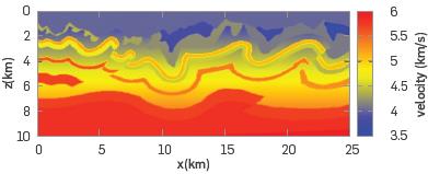
Figure 2 The Canadian Foothills. This is a sub-sampled version of size 334x200. The original model size is 1169x1000. 

Experiment 1. In this case we used the topography profile of the Foothills model and replaced the original velocity values for a 2-layer model of constant velocity separated by a straight horizontal interface. This numerical experiment is intended to examine the details of the image obtained with RTM in Riemannian coordinates, which is a good starting point. The interface of the 2 layers is located at 5 km depth. The velocity of the upper layer is 4 km/s and the other is 5 km/s. The step sizes for these grids were dx = 0.075 km and dz = 0.05 km. The time step is 0.001s. The source used is a Ricker pulse with a central frequency of 6 Hz. We use 24 shots to cover the model.

The RTM result for the Riemannian algorithm is shown in Figure 3, while the result of the purely Cartesian version is shown in Figure 4.

Figure 3 Riemannian RTM image for a two-layer model with an upper boundary that corresponds to a section of the full Canadian Foothills model. 

Figure 4 Cartesian RTM image for a two-layer model with an upper boundary corresponding to a section of the full Canadian Foothills model. 

The upper curved border should be smoothed in the Riemannian case as the calculation of the metric tensor implies the computation of the derivative along the surface topography. We also explored the application of cubic splines or Bezier curves to the mountain profile expecting to get more precise results, but these were not much better. The mountain profile of Figure 4, on the contrary, is the exact profile of the mountain in the sub-sampled Canadian Foothills model. Comparing Figures 3 and 4, it is evident that the RTM image for the Riemannian coordinates produced a reflecting interface more irregular than the image of the Cartesian case. On the one hand, this is caused by the distortion of the seismic waves due to effects of numerical dispersion, and, on the other hand, due to the fact that in a curved mesh it is harder to represent the straight line corresponding to the plane interface. The Cartesian image shows some shadows (or artifacts) in places away from the interface (the interface is the only region where we expect to see something in this case). These artifacts can be produced for the multiple wave reflections over the border of the mountain. As in the Riemannian scenario the border is smooth, it is obvious to expect less artifact there.

Experiment 2. This numerical experiment also involves the Canadian Foothills velocity model shown in Figure 2 although using its full complex inner structure. This model should be transformed into the Riemannian domain, i.e., the computational domain, using the transformation rule given by Equation 1 and Equation 2. The transformed model is shown in Figure 5.

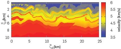
Figure 5 Transformation of the Canadian Foothills model into the computational domain. The topography profile of Figure 2 is mapped into a horizontal line and all the points below are deformed in a similar way. 

The RTM image for the Cartesian case is shown in Figure 6, and the image for the Riemannian case is shown in Figure 7. The values of dx, dz, dt, frequency and the size of the grid are the same that we used for Experiment 1.

Figure 6 RTM image for sub-sampled Canadian Foothills velocity model in the Cartesian scenario. This is a subsampled version of size 334x200. 

Figure 7 RTM image for sub-sampled Canadian Foothills velocity model in the Riemannian scenario. 

Comparing the Figures 6 and 7, there is no visible image improvement in the Riemannian scenario. The near surface details of the Cartesian image seem to be better and the amplitude of the image of the reflector is more continuous Furthermore, it is not true that the curved grid is more suitable to describe scenarios with rugged topography as the mountain border in the Riemannian domain is not the original one but a smoothed version. The resolution of the reflectors in Figures 6 and 7 is not good because the spatial sampling used in this experiment implies that the frequency of the Ricker pulse must be low, so fine structures cannot be well resolved.

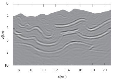
To improve the resolution of the reflectors, we applied the Cartesian RTM algorithm to a section of the full model (no subsampled) which is shown in Figure 8. In this case the sampling interval in the horizontal direction is dx=0.015 km and in the vertical direction it is dz=0.010 km. Since these parameters are smaller than those used in Experiments 1 and 2, a higher frequency is used (25 Hz). The result is shown in Figure 9. It was not possible to obtain an analog image using the Riemannian scenario because for this set of parameters the modelling not was not stable, and the time sampling required for a stable modeling was too small and impractical.

Figure 8 A section of the Canadian foothills model. 

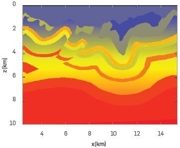
Figure 9 RTM image for the model shown in Figure 8. This result was calculated with the Cartesian algorithm. 

POST-PROCESSING MIGRATED MODELS

The cross-correlation imaging condition produces, in migrated mages, spatial low-frequency noise, (artifacts). This is caused by the superposition of head, diving and backscattered waves. These artifacts can hide important details in the image and affect its (image) interpretation.

The reduction or elimination of artifacts has been widely studied and several techniques have been proposed.

We use the Laplacian filtering proposed by Youn and Zhou ^[14] and the Laguerre-Gauss filtering described in Paniagua et al. ^[15]. We compare and analyze the images obtained by the these filtering methods.

The Laplacian filtering has been used for an edge enhancement in digital image processing ^[16].

It also shows good attenuation of the migration artifacts. This technique has two major effects: (1) it removes the low-frequency information and (2) it increases the high-frequency noise ^[17],[18] Laguerre-Gauss filtering is a post-processing technique that avoids the high frequency noise and reduces the artifacts due to its property of being an isotropic bandpass filter ^[15],[19].

To show the effects of the Laplacian and Laguerre-Gauss filtering in the migrated image, we applied them to the synthetic dataset. Figure 10 shows the comparison of the results obtained by applying both filtering techniques.

Figure 10 (a) RTM image plus Laplacian filtering (b) RTM image plus Laguerre-Gauss filtering. 

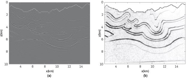
Figure 10a shows the image obtained by applying the proposed method using the zero-lag cross-correlation imaging condition and the Laplacian filtering. The low-frequency artifacts are reduced but in different parts there is some high frequency noise.

The seismic image is improved by applying the Laguerre-gauss filtering (Figure 10b). The artifacts are significantly reduced, the structures are more defined and enhanced.

Some details are improved in the image using the Laguerre-Gauss filter. It should be noted that the artifacts in shallow parts and near the reflective event are significantly reduced and the subsurface structure is further defined and enhanced. The Laguerre-Gauss filter can enhance any small changes in the seismic image and preserve the true location of reflections.

CONCLUSIONS

The images obtained by the RTM algorithm in Riemannian coordinates for the sub-sampled velocity model are not better that those obtained in Cartesian coordinates. When we used the Canadian Foothills model without subsampling, the Riemannian stability condition implies a very small and impractical time step, so we only obtained the RTM in this case for the Cartesian algorithm, without finding any advantage in the Riemannian coordinates formulation

The numerical experiments show that the time step implied by the stability condition depends strongly on the degree of smoothness of the mountain profile. To obtain time steps that are suitable for calculation, we must represent the topography with curves that do not pass exactly through each point of the true profile, so the main objective of the Riemannian method is not achieved.

Different transformations from the physical domain to the computational domain imply different metric tensors and, in turn, different limits for the time step necessary for stability purposes.