


 English (pdf)
 Article in xml format
 Article references
 Send this article by e-mail
 Cited by SciELO
  Cited by Google
  Similars in
SciELO
Similars in
SciELO  Similars in Google
 Permalink
1. INTRODUCTION
The following work is intended to solve the bidimensional elastic wave equation in a high performance computational architecture; this process is commonly used in high cost computational algorithms such as RTM and FWI to infer, by means of seismic studies, the properties and location of the geological structures with hydrocarbon content in the subsurface. Essentially, seismic modelling is the construction of computational simulations to show the diverse reflection and refraction phenomena of energy in the subsurface. The key idea is to simulate the acquisition and reproduction of some synthetic records. This technique is a valuable tool for interpreting field seismograms and solution of seismic inversion algorithms.
Seismic imaging uses reflected energy to build an image of subsurface in order to investigate the underlying structure and stratigraphy. These can be compared with seismic records to review data such as layer thickness, type of rock, fault formation, fracturing and salt deposits. As these simulations demand numerous computational resources, it is necessary to use high performance computation that enables carrying out experiments and get results in the shortest time possible.
Similar work has been conducted in the area. Komatitsch, Erlebacher Goddeke and Michea [1] discuss a formulation based on finite elements for the tridimensional wave propagation in an anisotropic media. Weiss and Shragge [2] developed wave field models in 2D and 3D in an anisotropic elastic media, resolving the equations with finite differences by using a regular grid, implemented in a massively parallel CUDA-based programming setting. Das, Chen and Hobson [3] in the study of seismic events, generated synthetic seismograms solving a tridimensional wave equation in elastic media using the pseudo-spectral method, parallelized in GPU units. The contribution of this work is the modelling of bidimensional wave propagation in elastic media, using a staggered grid to reduce the numerical dispersion. It is also implemented on a GPU-based structure and it is compared with the CPU implementation of several cores.
The document is organized as follows: the phenomena associated with the transmission of energy in P and S waves, together with the computational solution considerations are described in section two. Section three shows aspects related to the implementation while the results obtained are addressed in section four and the conclusions.
2. THEORETICAL FRAMEWORK
PHENOMENOLOGY OF P AND S WAVES ENERGY TRANSMISSION
The energy of a seismic wave is transmitted in an isotropic elastic medium as two types of waves, those called P Waves, where the vibration of particles is polarized in the propagation direction and the S Waves, where the vibration of particles are polarized perpendicular to the wave propagation direction. The seismic modeling is a computational technique that allows to build simulations of energy reflection and refraction phenomena in the subsoil. An initial approach of the modelling for wave propagation in a medium is to consider the equation as if it were an acoustic medium; however, this approach does not consider the medium density variations, which is not the case in seismic data acquisition. To carry out the modeling process, the expressions for deformation in an elastic medium must be specified, to then arrive to the wave propagation formula in such medium.
The elastic dynamics has an energy conversion property when the wave front finds changes in the medium properties. This results in a longitudinal wave field (P) in the direction of the wave propagation direction, which modifies the volume of the medium by exerting compression, and a rotational wave field (S) which propagates transversal to the propagation direction. The interaction between these wave fields result in a dipolar behavior: the more P wave field amplitude the least S wave field amplitude and vice versa. To model these propagations, the internal forces of resistance to compression must be considered, which can be expressed through the stress tensor. At the same time, these forces give rise to acceleration and velocities in the medium, which are obtained synthetically through simulation or through seismic data acquisition. The ratios of velocities and stress tensor result in a differential equation system in partial derivate proposed by Virieux [4], and his solution proposal through finite differences by Fornberg [5] result in an explicit numerical scheme shown in equations 1 to 5.
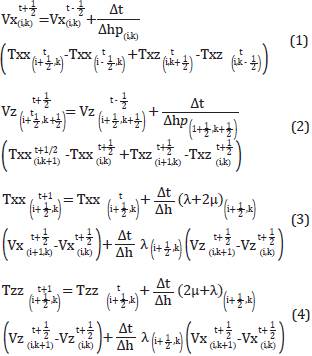
Where Vx and Vz are the velocity fields in the horizontal and depth axis, respectively. Txx, Tzz and Txz are the tensions on planes xx, zz and xz respectively. The t variable is the time integration index, l is the coordinate index on axis x and k is the coordinate index on axis z. The grid steps over time and on spatial axis x and z are Δt and Δh respectively. The μ y λ values correspond to Lamé coefficients. The stability condition is more restrictive dueto the presence of shearing velocity Vz given by formula 1 as proposed by Bamberger, Chavent and LaiLLy [6], considering that Δx = Δz.
When these equations are modelled and both wave fields are obtained and these get close to an interface given by the change of medium, part of the energy is reflected and the other one is refracted. When a P wave field is reflected, there will be a new P wave field and an S wave field. This is also the case with refracted energy. This phenomenon is known as conversion of the P-S energy and is shown in Figure 1.
In order to prove this computational scheme, a solution of the acoustic and elastic equation is presented in a three-layer heterogeneous model whose dimensions are 4 km distance and 2.4 km depth for axis x and y, respectively. The experimental parameters are shown in Table 1.
Table 1 Parameters of a three-layer heterogeneous medium for testing the reflection and refraction in the acoustic and elastic media.
Considering that the source is located within the model and on the surface (x = 2km, y = 0km), all events occurred during the simulation of 1.7s are registered, rendering the results shown in Figure 2b for the simulation in the acoustic medium and the results are shown in Figures 3a and 3c for the simulation in the elastic medium. With respect to the acoustic simulation, the expected response is the direct wave and to additional reflections from the 2 interfaces for the thee-layer model. As regards the elastic simulation in both registers Vx and Vz, there are more than 2 reflections due to the Energy conversion.
Figure 2 Records for a three-layer model with data presented in table 1. (a) Vx con onda en medio elástico (b) Presión en medio acústico (c) Vz en medio elástico.
CONSIDERATIONS ABOUT THE COMPUTATIONAL SOLUTION.
THE PERTURBATION SOURCE
As regards the perturbation source, the Ormsby filter is used which consists in a trapezoidal zero-phase wavelet for its frequency response. In the seismic exploration area, this type of wavelet is useful as it is similar to the acquisitions with vibrator trucks, as these allow for observing low or high frequency noise while the wave energy dissipates as it propagates in length and depth. The frequencies in this case are f1 f2, f3, f4:5,10,60 and 80Hz respectively where f: is the low cutoff frequency, f2 is the low-passing frequency f3 is the high-passing frequency and, finally, f4 is the high cutoff frequency. Figure 3a shows the response of a homogeneous medium to an Orsmby source in an acoustic medium, and Figure 3b and 3c represent the solution of the wave equation in an elastic medium. Two perturbations are identified in these figures, one of them represented by a P wave velocity field, and the second one is the medium response given by the shear- velocity. Lastly, Figure 3d and 3e show the response in the time domain and in the frequency domain, respectively.
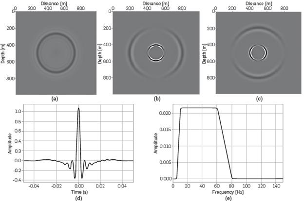
Figure 3 Simulation of the response of the medium in pressure and velocities of an Ormsby wavelet, (a) Response of pressure field to an Ormbsy wavelet in an acoustic homogeneous medium (b) Response of the Vx field to an Ormsby wavelet in an elastic homogeneous medium (c) Response of the Vz field to an Ormsby wavelet in an elastic homogeneous medium (d) Response of the Ormsby Wavelet [5-10-60-80]Hz in function of the time (e) Frequency response of the Ormsby Wavelet [5-10-60-80]Hz
MANAGEMENT OF BOUNDARY CONDITIONS
The absorbing boundary conditions are desirable to eliminate artificial reflections produced when the energy propagation simulation reaches the limits of the implementation matrix, which size is finite. In theory, the wave fronts propagate toward infinite while energy dissipates, but actually the mesh where the simulation takes place has logical limits, which generate false reflections. There are several proposals to solve this problem. One proposal that has rendered good results if that of the Perfectly Matched Layer (PML) by Berenger [7], whose initial implementations were done with electromagnetic simulations. In the continuous limit it has been confirmed that the PML has no reflections, regardless of the incidence angle and the frequency established by Zeng and Liu [8] and there are no instability problems related to the models where the ratio Vs/Vp is less than 0.5 as proposed by Mahrer [9] and Stacey [10]. The PML region is located near the computational Limit as shown in Figure 4. Following a Cartesian plane, the 2D elastic wave equation can be expressed as a first order differential equation system in terms of velocity and stresses in the particles and its implementation can be formulated with a simple variable division procedure in the spatial domain, where one component is tangential to the field and the other is orthogonal.
Figure4. Matrix scheme near the computational limits. The dark region is an area of the grid where false reflections are attenuated.
To prove the numerical validity of the PML, the experiment shown in Figures 5a-5h was performed. A source is located in the position (300,800) [m] and all events in the position (300,800) [m] are registered, which is marked on the guide intersection lines on Figures 5a-5c and 5e-5g. The parameters used in the PML are 20 points and an amortization coefficient R=0.0001 showing the following results in Figure 5.
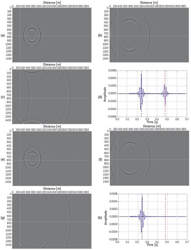
Figure 5 Experiments to test behavior in the grid boundary using the PML. (a) Simulation time 0.2[s] (b) Simulation time 0.3[s] (c) Simulation time 0.5[s] (d) Record of incident and reflected wave by the boundary, without using PML. (e) Simulation Time 0.2[s] (f) Simulation Time 0.3[s] (g) Simulation Time 0.5[s] (h) Record of incident and reflected wave by the boundary, using PML.
It is noted that when using the PML there is no wave amplitude reflected and, therefore, there will be no reflections due to computational boundaries.
BOUNDARY INSTABILITY SOLUTION.
When dividing the velocity and deformation components on tangential and orthogonal elements to apply the PML, there is one specific case in which this form of wave attenuation shows Instability and that is when there are shear-velocity components Vs=0 and Vs>0: which Is common when reproducing offshore seismic acquisitions. The next experiment Is a simple geological model where the upper Layer Is water and the lower layer Is a solid Such instability can be observed in the experiment shown In Figures 6a to 6f.
Figure 6 (a) Vx field at t=0.04[s] (b) Vx field at t=0.1[s] (c) Vx field at t=0.2[s] (d) Vz field at t=0.04[s].
To solve this instability Issue, It was proposed to use a gaussian filter only on the shear velocity values within the PML zone, so that In places where the transition Vs=0 (water) and V s >0 exists, it would be as smooth as possible. Keeping this in mind, the same experiment was reproduced, obtaining the results shown in Figures 7a to 7f.
3. EXPERIMENTAL DEVELOPMENT.
Nearly all new processors work on the development of computational architecture based on central processing units (hereinafter CPU) where the processor received instructions from the memory that are subsequently decoded to finally execute the instruction and store the result again in the memory.
The distributed computation, commonly called cluster computing is a good way to solve large applications demanding high computational costs. This notion consists in taking a given number of computers and connecting them in a network with the potential of enhancing several times the computational performance to solve the application. However, it should be taken into account that the network velocity is a limiting factor.
The architecture in a modern graphic processing unit (GPU) is no different than a multi-node scheme. The GPU has a finite number of multiprocessors (SMs) that are very similar to the cores in a CPU. A modern GPU is connected to a computation system by means of a PCI port that is much faster than a network connection. This way it would be possible to have better performance, without being limited by the transmission of the results.
The notion behind better performance in GPU is that these processing units comprise a processor array (SM), each with N cores. The more SMs in the GPU, the more tasks processed simultaneously In each SM there are several SP (units that have an array of a series of processing cores and special function units). Each SM has access to a set of records that have the same velocity than an SP unit, where each SP has a shared memory, which Is accessible for each SM.
COMPUTATION SYSTEM USED
In order to compare the efficiency of computation architectures, some implementation tests were performed on different architectures. With respect to CPU tests, these were performed in the next processing node belonging to the research group of Connectivity and Processing of Signals (CPS) of Universidad industrial de Santander.
The programming environment used was CUDA (Compute Unified Device Architecture), which is an extension for programming Languages such as C, C++, FORTRAN, Python and others; it supports the graphic processing units to execute applications created in those Languages. The CUDA language extensions follow a heterogeneous programming concept. The foregoing means that to execute applications in a graphic processing unit, the main program must be launched by the processor and then the functions that are to be executed in parallel will be launched in the GPU. These functions are executed in graphic processing units.
IMPLEMENTATION IN CPY AND GPU COMPUTATIONAL ARCHITECTURE.
For implementation in all CPU cores, the OpenMP programming extensions were used, which enables dividing the programming cycles (for) in the number of threads of the processor. This programming model is based on shared memory systems. This means that each thread can access the whole memory reserved for the application, carry out any operation and write thereon. It is, therefore, fundamental to make a distinction between private and shared variables.
The Marmousi elastic model will be used, as standard, in all tests, which dimensions are 13601 x 2801. This model has a spatial interval Ah of 1m and due to the small memory of the GPU, the idea is to simulate only 1.1 seconds of a seismic acquisition. In general, a seismic acquisition implies 4 to 6 seconds recording and, therefore, the use of asynchronous executions and memory copies is proposed further below in order to fully simulate a seismic acquisition in the GPU, with the limit not being the memory of the GPU but the RAM memory of the whole computation system to thus obtain faster executions. All operations, both in CPU and GPU, were done with double precision arithmetic.
There are two basic forms of dividing the work load in a CPU that is, using static or dynamic distributions. The experiment was conducted trying both forms, having chosen the dynamic distribution as it is closer to the ideal performance, as can be seen in Figure 8.
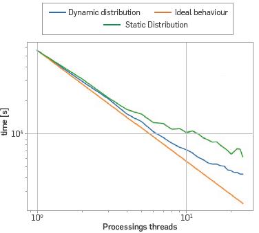
Figure 8 Solution of the elastic wave equation in the Marmousi model, with a simulation time of 1.1[s] through static and dynamic distribution. Time using dynamic distribution with 1 core t1=57023[s], Time using dynamic distribution with 24 cores t 24=4325[s].
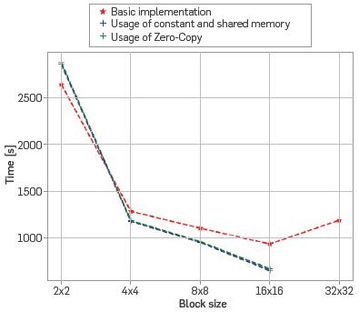
With respect to the implementation in the GPU, 3 versions were issued. The first one is a simple coding where all variables are stored in the global memory of the GPU. The second one uses the constant memory and the shared memory of the GPU to accelerate even more the calculations, and a third version called (Zero-Copy) where even using the shared and constant memories, asynchronous copies between the GPU memory and the CPU memory were made in order to simulate in the GPU a full acquisition without being restricted by its small memory.
Equal to the code execution in the CPU, the time to be simulated is 1.1[s) and for each version the intent is to change the block size to determine the size with the shortest execution time. The sizes of the blocks used were 2x2, 4x4, 8x8, 16x16. The test using 32x32 thread blocks was possible only by using the global memory (version 1 of the code), as the GPU architecture has restrictions related to the use of the shared memory with blocks containing 1024 threads or more.
The best performance is obtained by using 16x16 blocks, regardless of the copies being synchronous or asynchronous, as observed in Figure 9, even though the additional time of the kernel (core) with asynchronous copies is approximately 20[s] more.
4. RESULTS ANALYSIS
EXECUTION LIMITED BY LATENCY OR MEMORY
After knowing the size of the ideal block to obtain the shortest execution time, it is assessed if this type of kernel is limited by latency or by memory. A latency problem is that the instruction to be executed by the thread has so many operations to carry out that it limited by the clock velocity of the thousands of cores in a GPU. On the contrary, a memory problem issued is how dependent is the instruction on uploading all values from the memory to then perform the respective operation.
Ideally there should be a homogeneous performance and as high as possible between the operation functions and the memory transactions. Using the Nvidia Visual Profiler (NVVP) [11] tool, it is possible to evaluate the overall performance of the application execution in the GPU. To such end, version 1 of the code is compared vs. version 3, where the shared memory and the constant memory in the kernel are used, as this helps to a faster uploading of the values, thus increasing the velocity of the execution. When using this type of memory, in practice the preloading of values for processing the elastic wave equation improves by nearly 10 per cent points (55%) the response of the GPU with respect to latency and memory transfer.
A more detailed analysis of memory performance can be observed by analyzing the throughput of each implementation as observed in Figures 10a, 10b, 11a and lib.
Figure 10 (a) Percentage of use of computation functions and GDDR5 memory using version 1 (global memory) (b) Percentage of use of computation functions and GDDR5 memory using version 3 (zero copy + const_mem + shared_mem)).
USAGE OF THE GPU
The usage factor of the GPU can be obtained by evaluating the kernel with the NVVP [CUDA, 2017] tool, in addition to other significant variables for assessing the kernel performance such as:
To visualize kernel results, a comparison was made between basic implementation in a GPU and implementation using asynchronous copies with shared and constant memories, which responses are shown in Figures 12a and 12b. As can be observed in the figure, a detailed use of the various memory hierarchies provided by this GPU architecture can increase by nearly 20 percent points the Occupancy variable, which shows how busy the GPU is calculating with active threads. Having values in the shared memory enables having more active blocks, as these will not have to wait for obtaining values from the global memory. Another aspect to analyze is the behavior of records with respect to active threads. When feeding the shared memory, the records upload the additional values; therefore, it is ideal when these are integer numbers and multiples of the number of threads that exist in a warp. When using the shared memory and uploading the additional values for calculating the eighth order stencil, this translates in the record access to the threads being as aligned as possible. This ratio can also be seen in Figures 12c and 12d under the SM occupancy heading.
Figure 12 (a) Variable Occupancy per SM (utilization per multiprocessor) in the implementation of the code using the global memory only (b) Variable Occupancy per SM (utilization per multiprocessor) in the implementation of the code using the zero-copy + mem const + mem shared, (c) Usage of records per thread, per block and block limit using the global memory (d) Usage of records per thread, per block and block limit using zero-copy + mem cons + mem shared.
OPERATIONS BY TIME UNIT
One of the most relevant measures in the high performance computation setting is the number of operations required by a certain computation unit to fully complete a task. This unit is known as flops. The last analysis proposed is to record operations by time unit required by the CPU to carry out the task and the necessary operations in each of the 3 implementations in the GPU, resulting on that shown in Figure 13.
It is evident that using a GPU to solve this type of simulations is much more efficient than using a CPU, but if the performance is to be even better, the code that was developed should be restructured to use concurrent kernels.
CONCLUSIONS
The bidimensional wave equation in isotropic medium was solved by means of finite differences in the temporary domain in two computation architectures, with programming shared memory applications. When working out this equation, the stability of the various test models was evident.
Furthermore, the Ormsby wavelet set in the tests is a type of signal commonly used in synthetic experiments, as it enables obtaining response of the medium in a wide range of frequencies.
A comparison was made with respect to the execution time between two different processing architectures, such as a CPU and a GPU. As regards the CPU, its processing resources and memory were used as much as possible, using the OPENMP application programming interface to use all the processing cores. Several simulation experiments were performed for comparing their performance as related to execution times and floating point operations. It is concluded that the execution of the modelled process is more efficient when using the implementation in GPU (use of zero-copy with shared memory and constant memory) vs. the implementation in a 24-core CPU, as it is almost 12 times faster. Thus, a GPU is an alternative to carry out fast and efficient calculations.

