INTRODUCTION

Simplified models for transient flow in pipes have been developed from the equations used to study transient phenomena such as water hammer ^[1]. The model consists of equations of mass conservation, momentum and energy for average properties in the cross-sectional area for a compressible fluid, as is proposed in ^{[8], [9],} Transient two-dimensional models, such as the one proposed in ^{[5],[10],[14],} can provide important understanding regarding the transient pipe flow phenomena. Nevertheless, computational cost associated to spatial discretization procedures makes the analysis impractical in cases where pipe length is much greater than the diameter. In those situations, a one-dimensional approach is sufficient to capture relevant aspects of transient heavy crude flow ^[4]; for instance, estimation of the inlet pressure that starts up the flow or determination of the maximum pressure foran imposed inlet flow rate ^[15].

Davidson et al. ^[2] developed an algebraic model based on control volumes to model the behavior of paraffinic crudes in restart situations with water or oil injection, based on the model designed by Cheng et al. ^[3] which improves formulations developed in ^[11],[12] by including compressibility and time dependent Bingham constitutive equations. The authors find that the viscoplastic behavior and compressibility of the paraffinic crude is a determining factor in restart and restoration time of operational conditions, Vinay et al. ^[4] solves differential and one-dimensional mass and momentum balances for a viscoplastic fluid (Bingham Plastic). The model developed is based on a two-dimensional model for barely compressible and viscoplastic flow ^[5]. The authors state that the use of one-dimensional models is more appropriate for applied cases, considering the aspect ratio of the pipes and the computation times. In addition to establishing relevant dimensionless numbers for the restart of crude oils, Vinay et al. ^[4], solve mass and momentum balances, finding the stabilization times for three important scales: compressible diffusion proportional to the dimensionless compressibility (ß*), acoustic propagation proportional to the product of ß* and Reynolds number (fie) and viscous damping proportional to fie. With a similar model but reducing dimensionality to a 1.5D approach, Wachs et al. ^[13] and Ahmadpour et al. ^[16] obtain results as accurate as the two-dimensional case, reducing computational time to a fraction of the 2D case. De Oliveira et al, ^[6] solve the aforementioned equations using the finite volume method, as proposed by Patankar ^[20], to describe the behavior of paraffinic (viscoplastic) crude in restart situations as a function of the dimensionless numbers fie, ß*, aspect ratio (5), dimensionless gravity and the Bingham number (B). The authors conclude that with a lower fie, the time of restoration is greater, low values of ß* produce greater oscillations in the pressure increasing the restoration time, and the dissipation of the pressure peaks is higher in horizontal tubes than vertical. Using a similar numerical method, Sun et al. ^[17] compare different rheological models for waxy crude oil emulsions, concluding that the model proposed by Teng and Zhang ^[18] adequately describes yielding phenomena Liu et al. ^[7] includes the energy conservation equation in a one-dimensional differential model of transient flow in pipes based on the mathematical description of the phenomenon presented in ^[1] By means of the characteristics method, the authors find restoration times of operational conditions, taking into account the thermal scale, which is significantly higher than the scales mentioned above, where only isothermal effects are considered. Based on this method Li et al. ^[19] developed a computational tool to predict temperature drop after shutdown and pressure and flow rate during restart.

The model used to obtain the results presented in this article is made up of the partial equations presented by Liu et al. ^[7] Although this model does not consider the viscoplastic behavior of paraffinic crudes, it can be used as a first approximation to the transient behavior of non-isothermal heavy crudes, since the variation of viscosity in terms of temperature is considered by the friction factor. Therefore, the main contribution of this paper is the implementation of a thermohydraulic model to simulate transient fluid flow and heat transfer in heavy crude pipelines considering the fact that, to the best of the authors' knowledge, numerical results for heavy crude pipe flow regarding velocity, pressure and temperature have not been obtained. Recent research on heavy crude fluid dynamics is mainly focused on experimental thermal shrinkage ^[22] friction reduction ^[23] and rheological behavior in terms of additive concentration ^[23],[24], water cut ^[25] or a lighter crude content ^[26], The proposed model could include non-Newtonian behavior, thermal shrinkage and temperature dependency of transport properties. However, this work is focused on introducing a modeling methodology to simulate heavy crude pipeline flow, widening the applicability of the model implemented in ^[7].

In the next section, an explanation is provided regarding the model, as well as the dimensionless parameters derived from the conservation equations of mass, momentum and energy. In the Last section, results are presented for a validation case as well as additional cases where, among other quantities, the crude properties (viscosity and density), length and topography of the pipeline and operation parameters of the pipeline are varied (operation flow rate). Everything mentioned previously was Included in order to find relevant results for hydraulic and thermal restoration time, as well as the maximum pressure allowable in the restart process.

THEORETICAL FRAME

Based on the differential balances in terms of average quantities in the cross-sectional area of the pipe, it Is possible to obtain a mathematical model whose solution represents the behavior of relevant variables in time and axial direction (z coordinate). The mass conservation equation can be expressed in terms of pressure (P) and the average velocity In the axial direction (V) according to equation (1), considering the compressibility effects of crude, whose relevance is given by the shrinkage exhibited by the crude oil in stop conditions, given the cooling ^[4],

The linear momentum conservation equation (2) Includes terms of inertia, compression, friction and gravity. The effect of the viscosity of the crude oil is given by the coefficient of friction, which is also found as a function of the radius (R), the density (ρ), the velocity and the roughness from an explicit approximation of the Colebrook-White equation. Friction factor is related to temperature by means of the Reynolds number, which is a function of viscosity An experimentally-fitted exponential equation is used to describe viscosity behavior In terms of temperature. The angle of inclination of the pipe (θ) is found by interpolation of the pipe's topographic data, which Is part of the input data for transient state simulation and, in general, can change with the distance along the pipe z.

The conservation of energy In the crude inside the pipeline is given by the expression (3) that Includes terms of temporal and spatial variation of enthalpy in terms of temperature (T), compressibility, viscous dissipation and heat loss by walls. For simplicity, the thermodynamic properties, both In this and in the other equations, are considered constant at a reference temperature. The overall heat transfer coefficient (U) is obtained by an analysis of equivalent thermal resistance in the crude-pipe-soil system, considering the conductivities of each material and the conduction resistance between the pipe and the ground.

The Initial conditions correspond to a crude oil at rest (V(z,0)= 0) brought underthe hydrostatic pressure as a function of the relative height (h-h₀):

The Initial temperature distribution will be an input function to the model and defined according to the stop time. Two types of boundary conditions can be imposed for velocity and pressure. The first corresponds to Input pressure, i.e.

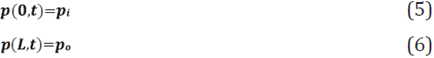
This condition is applied in the case that one wishes to know the behavior of the velocity in time and the operation flow rate in a steady state. The second possibility is a known operating flow condition (Q):

This condition, together with the output pressure condition (6) is used to ascertain the transient behavior of the pressure in the restart process, as well as its maximum value and steady state. Considering the hyperbolic and non-linear nature of the system of governing equations, a scheme of finite differences (MacCormack-type, explicit second order) Is used for their spatial and temporal discretization. This numerical scheme is a two-step method with a first step (predictor) In which Intermediate pressure, velocity and temperature are found from previous (or Initial) values. The second step (corrector) uses the intermediate variable values in order to obtain a better approximation and complete time step calculations. More details about the method employed can be found in ^[21]

DIMENSIONLESS NUMBERS

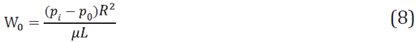
It Is possible to obtain a group of dimensionless numbers from the conservation equations (1-3) according to the strategy presented in ^[4]. Among other properties, the dimensionless numbers are expressed in terms of the characteristic velocity, whose definition depends on the type of boundary conditions. In the case of known inlet pressure, it is defined as:

For the second case (known operating flow), the characteristic velocity can be expressed as the average steady state velocity or:

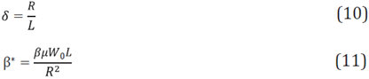
From mass conservation equation, two dimensionless parameters are obtained, the aspect ratio of the pipe (δ) and the dimensionless compressibility (𝛽*) which can be expressed, respectively, as:

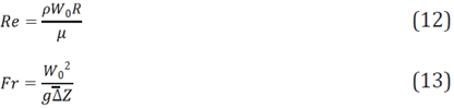
The dimensionless momentum conservation equation is a function of Reynolds and Froude Numbers:

The average height difference can be evaluated approximately as It is Important to note that, in this case, the sign of the Froude number must be considered in a similarity analysis. Another important dimensionless number related to the momentum is the friction factor of Darcy-Weisbach. However, this, for calculation purposes, depends on the Reynolds number and the relative roughness of the pipe, given by:

Therefore, assuring similarity of Re and e would result in the same value of the friction factor. Regarding the equation for the dimensionless conservation of thermal energy, It is possible to obtain a modified Eckert number (Ec’) since it is not In terms of the temperature of the surrounding environment but in terms of the temperature of the crude output (To). The Eckert number establishes a relationship between the kinetic energy of the stream and the change of internal energy In the pipeline and is given by equation (15). Additionally, a relationship is obtained between the heat transferred from the crude oil and the specific heat thereof, known as the Stanton number (St), equation (16)

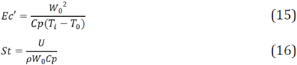
Finally, it is possible to express the contribution of thermal energy by compression/expansion In terms of a relationship between properties of the oil identified in this document, as a relationship between isothermal compressibility and thermal expansion (RCE) given by the following equation:

The previous dimensionless numbers will be relevant in scaling processes for situations of crude oil flow in pipe in transitory state. At the time of evaluating results it will be important to express relevant variables in dimensionless terms. This is because, according to the scales used to obtain the dimensionless parameters, independent dimensionless variables are defined, such as time and distance, given by equations (18) and (19), and dimensionless dependent variables such as pressure, velocity and temperature, expressions (20), (21) and (22), respectively.

Equations (1), (2) and (3) are solved for the initial and border conditions mentioned for different cases of the re-start process on an industrial scale. In the following section, one of these cases is used to perform the validation of the numerical scheme. Subsequently, results for different cases are presented and important output variables are calculated such as approximate times of hydraulic and thermal stabilization, and maximum pressure at restart and steady state.

3. RESULTS

In order to validate the numerical procedure to solve the governing equations in terms of time and axial distance, a real reference case is used, of which the following data are known, in addition to the topography and the calculated and verified pressure and temperature distribution In the steady state:

Q = 200,000 BPD

T_i = 170 °F

P_i = 1000 psig

P_o = 243.5 psig

k_T = 28 BTU/hr ft °F

k_S = 1.3 BTU/hr ft °F

h_T = 1 m

T_∞ = 75 °F

ε = 0.0018 in

°API _@60°F = 16

μ _@86°F = 672 cSt

μ _@170°F = 74.28 cSt

The reference case corresponds to a pipeline section with a length of 84 km, an external diameter of 24 in and a pipe thickness of 0.7 in An initial temperature distribution is assumed, given by the cooling of the pipeline at a stop in a lapse of 72 hours.

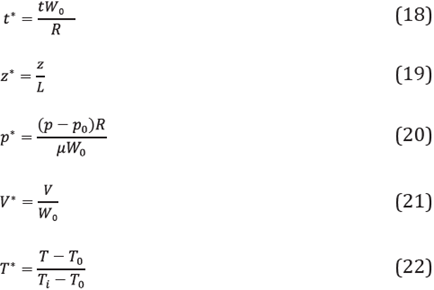
First, results are obtained for the case of known pressure at the pipeline inlet. From the results, two time scales can be differentiated. The first corresponds to the development or restoration of flow, which occurs, in this case, in a time less than 200 seconds. In this period, one sees propagation of the wave originating by the injection of crude oil at high pressure, setting the oil in motion along the pipeline, as can be seen from the pressure and flow profiles presented in Figure 1, where they show the distributions every 20 seconds. The small disturbances observed in the graphs are more related to the usage of a second-order numerical scheme when travelling waves are present, which is the case at small interval times after the restart operation

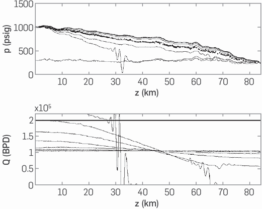
Figure 1 Pressure and flow profiles for validation case for t<200 s. Continuous lines correspond to calculated pressure and flow rate distribution in intervals of 20 s. Pointed lines indicate reference distributions at steady state. 

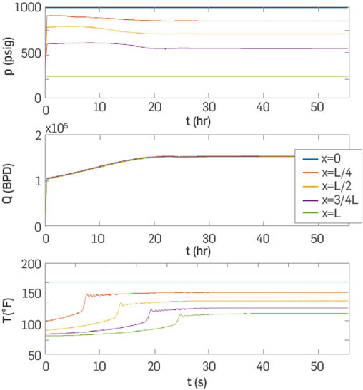
Figure 2 shows the evolution of the variables in some points of the pipeline, indicated by the label on it. The pressure increases considering a small gap between each point, according to the distance at the beginning of the pipeline. Similarly, due to the compressibility of the crude oil, the flow near the inlet exhibits a peak that decreases over time, to reach the same value for the whole pipeline. Negative flow rate values at points x=3/4 L and x=L before hydraulic travelling wave, are presented because of the aforementioned numerical overshooting problems. The period in which the same flow condition is reached in the entire pipeline will be referred to in this report as hydraulic reset time (t_rh). However, this value is far from being equal to the time in which the steady state (t_ee) is reached, since the temporary change in temperature occurs on a much higher time scale. It can be seen in the lower part of Figure 2 that the change in temperature is negligible in the period analyzed. To quantify changes in temperature and its effect on the other variables, it is necessary to obtain results for longer periods.

Figure 2 Evolution of average properties for t<200 s 

Figure 3 shows the pressure and temperature profiles for a time of 40 hours regarding the fact that time zero corresponds to the beginning of the restart procedure. For clarity, in the case of pressure, only the final profile is presented where a suitable estimate of the effects of the topography can be observed, with a maximum relative error of around 5%. As for temperature, the profiles obtained every 3 hours show an advance of the heating front that travels through the pipeline in the flow direction. When it reaches the end of the pipe, it still takes around 10 hours to reach the steady state, or in this case the balance between the heat generated by viscous dissipation and the heat lost by the walls of the pipe. In this case, the flow profiles are not presented since they do not offer additional information.

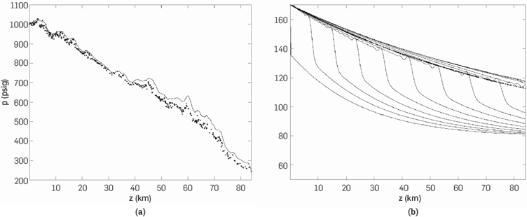
Figure 3 Pressure and temperature profiles for t<40 hr. Continuous lines correspond to calculated steady state pressure and flow rate distribution in intervals of 3 hr. Pointed lines indicate reference distributions at steady state. 

The increase in temperature along the pipeline causes a decrease in viscosity, which in turn causes a decrease in local pressure differences and an increase in operating flow, as can be seen in the graphs presented in Figure 4. In Figure 1, it Is possible to observe that both the pressure and the flow rate after 200s are far from the reference data, Indicated in the dotted graphs. After 40 hours, the steady state of the system is reached and the pressure and temperature are very close to the reference points (Figure 3). Figure 4 shows that, for time after restart, having appreciable changes in temperature depends on the position in tube length; for Instance, at x=L/4, a time close to 10 hours is needed to reach a temperature variation near to 50°C. The use of constant properties such as density, Isothermal compressibility, thermal expansion and the heat capacity of the crude and the thermal conductivity of wall and floor, cause an error in the results that Is reflected in the differences with the reference quantities, which in the case of the flow can reach up to 20% relative error. However, the solution procedure used can be employed for the comparative analysis of transient behavior in stop and restart situations for heavy oil pipelines.

Figure 4 Evolution of average properties for t<40 hours 

For the sake of brevity, the results obtained for the case of known flow boundary conditions are not presented since the values in the steady state are analogous to those obtained for the first case, taking into account that the differences with respect to the reference data fall on the pressure values.

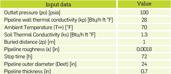
Results found by changing, among other parameters, operation volumetric flow rate, crude quality (viscosity and density) and pipe Length, are shown below. For the simulation of cases, a boundary condition for flow rate operation was established. The parameters that do not vary in the simulated cases are presented in Table 1 as input data. Among these, there are geometric aspects such as the diameter, roughness, thickness and burial distance of the pipeline, environmental conditions such as air temperature, properties such as the thermal conductivities of the pipe and the ground, and operational data such as the departure pressure and stop time; the Latter defines the initial temperature distribution along the pipeline.

Table 1 General conditions cases 

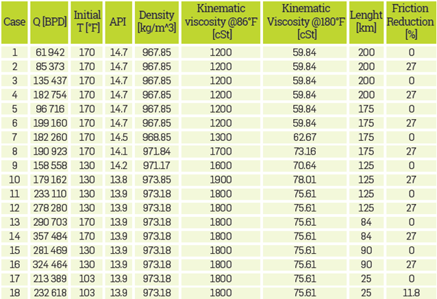
Each case is characterized by the aforementioned parameters. Table 2 shows the values of each of these variable parameters. Each case simulated relates to a variation of relevant properties with respect previous cases. For example, case two corresponds to case one varying the friction factor through a reduction of 27% of its original value. Case five corresponds to case three after changing pipe length, while case ten corresponds to case nine after changing the type of heavy crude oil and reducing the friction factor. Both the values of kinematic viscosity at different temperatures and the percentage of friction reduction make it possible to define the friction factor based on the viscosity model used and the direct application of the percentage on the total value of the friction factor. As it is shown in the table, the operational flow rate is changed in order to have comparable transient situations.

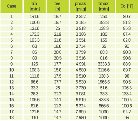
For brevity and ease of analysis, the results obtained are presented in Table 3 in terms of parameters relevant to the process of restarting the pipeline, as follows:

Table 2 Specific data for each simulated case 

According to the results presented in Table 3, the hydraulic restoration time is inversely proportional to the flow rate, i.e. the higher the flow rate, the shorter the hydraulic restitution time. In the case of the steady state time, the flow shows a similar relationship that is affected by the variation of other properties such as the kinematic viscosity of the crude, the initial temperature and the Length of the pipeline. The maximum pressure that is reported in the simulation during the re-start is proportional to the operational flow and the length of the pipeline. Regarding the percentage of friction reduction, it is clear that similar maximum pressures are obtained and hydraulic and steady-state restoration times are obtained for flow rates that differ by a percentage similar to the percentage of friction reduction; (compare cases 1 and 2, 3 and 4, 5 and 6, 7 and 8, etc). Since different parameters are varied in different cases, relationships between the other properties can be obtained by comparing results in terms of numbers and dimensionless variables.

Table 3 Results obtained for evaluated cases 

trh:hydraulic restart time, t_ee: stationary state time, p_max: maximum pressure at startup, t_max: maximum pressure time, T_o: crude oil outlet temperature

CONCLUSIONS