FWI ENGINE USED IN STATISTICAL EXPERIMENTS

We used a 2D representation of the subsurface, which is described by nz points along the z axis, and by nx points along the x axis, The distances between points are denoted by Δz, along the z axis, and by Δx, along the x axis. Every velocity model in this work is understood as a matrix of size NP= nz x nx. Each velocity element will be associated to the physical position (z _k ,x _l )=(k Δz,l Δx). From a computational perspective, the velocity model of the subsurface will be symbolized by a vector M = (c ₁ ,… ,c _NP ), where each value c. will be named as pixel. Each pixel of the vector M will be equal to a value of the velocity field, in an ordered way such that (k,l)→c _k+nz*l where the pair of indexes (k,l) will be understood as the position, in the computational mesh, of the pixel number k + nz* l. A number ns of sound sources, with coordinates (z _si ,x _si ) ∀ _i=1,…,ns , which generate the propagating waves are arranged. In all of our experiments, all sources are placed at the same depth z _si ∀ _i=1,…,ns . The sources are separated by a distance ds, and arranged along the x axis. Together with the sources, a number nr of receivers, separated a fixed distance dr between them, are placed along the x axis at coordinates (z _ri ,x _ri ) ∀ _j=1,…,nr . The observed data will be denoted by d _o .

The pressure field is symbolized with p(z,x,t). We used a Ricker's source function, g(t) = δ(z-z _s ) δ(x-x _s ), defined by with a dominant frequency f _d = 15Hz for all the cases studied in this paper. All the experiments were done by using a numeric solution to the acoustic wave equation.

With such solution we propagate the pressure field in order to get the synthetic data d _c . FWI makes a comparison between observed and synthetic data by iteratively minimizing an error function, denoted by E, estimated with a l ₂-norm. To easy the convergence of the method, a multi-scale approach has been employed.

The acoustic wave equation was solved by using the rapid expansion method (REM), [19], the pressure field is set at t= 0, for every point (z,x), as p=0 and ∂_t p=0. The gradients ∇E(M) were calculated by using the Adjoint State Method described in ^[20], In order to do the modeling of propagation of energy inside the finite nz x nx spatial domain, it is necessary to build artificial boundaries to simulate an infinite domain, and to avoid undesirable nonphysical reflections. To do this, we used Absorbing (Artificial) Boundary conditions.

The error function is evaluated for each iteration, as such evaluation is aimed at obtaining a good descent direction and making sure that the minimization procedure has been reached. We used the first Wolfe's condition, which is widely used with such procedure, ^{[19] ,[21]}.

where we used a ₁=10-3 and α₀=1.0. α_k is the step length that can be computed by a line-search algorithm [21], h _k is a search direction, usually determined by gradient methods, to find it we used L -BFGS. The minimization of the error function E(M) around the neighborhood of the initial model M ₀, is usually obtained through a Taylor's expansion of E(M). By equating the derivative, respect M, of such expansion to zero one gets the step descent ^[11],

where H _k ^-1 is an approximation to the inverse of the Hessian matrix, in the k-th step of the inversion, evaluated in M ₀ . The exact Hessian matrix, is usually neglected due to its large size and high computational cost ^[22].

METHODOLOGY FOR THE SETUP OF INITIAL MODELS AND FOR THE EXPERIMENTS

We will use as exact data sets: The Diffractor and the Marmousi velocity models, and these will be denoted as M _real , as shown in Figure 1. The term "real data" refers to exact data known in advance.

Figure 1 (a) Exact data set of Marmousi model, (b) Exact data set of the Diffractor model. 

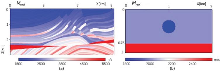
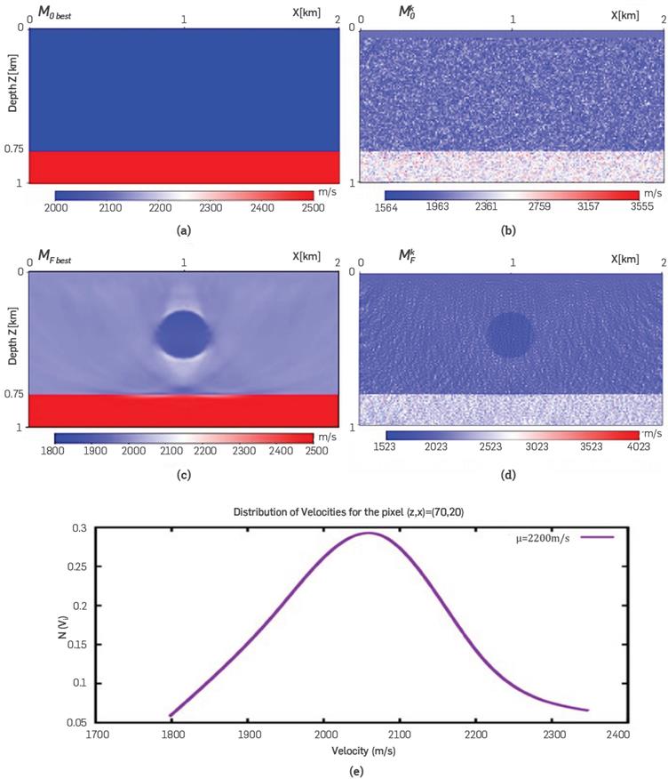
Figure 2 (a) The fiducial initial model, M _{Q best} , and its fiducial inverted model, M _{F best} , in (c). A perturbed initial model, for k=56, M ₀ ^k , and its FWI, M _F ^k , are displayed in (b) and (d), respectively, (e) It shows (quasi-normal) the distribution of velocities of the initial models cube for the pixel (70,20). 

Several initial models can be used as a starting point in FWI. This is supposing that fr ed from a smooth of the M _real of Figure la, Figure 3a contains letters A,B,C,D and E, pointing out several zones with relevant data from M _real which helps the convergence of the FWI, This fiducial initial model will be the initial model to obtain the best outcome from the FWI process.

Now, let be the collection of the nm possible starting models for the FWI, The ith pixel of the kth model, M ₀ ^k , will be Labeled by c ^k _0,i . If the information from the geophysical methods is consistent and coherent with the existing geological data, the nm aforementioned initial models may be similar but not identical, This similarity, considering that the non-linearity involved in FWI usually requires a good starting model, allows to argue, as one of our working hypothesis, that for a given fiducial starting model M _0best , the rest of possible initial models for a "successful FWI", may lie "close" to M _{0 best} .

An initial model M ₀ ^k (M ₀ ^k ≠M _{0 best} ) J will be considered "close" to the M _{0 best} , if for ith pixel c ^k _0,i ∈ M _{0 best} , the fractional difference with its corresponding ith pixel is smaller than or equal to a predefined tolerance perc, namely:

Thus, the perc value, allows for a discrepancy limit between the values of the pixels in M _{0 best} and any other possible initial model, Once a M _{0 best} has been chosen, the remaining nm-1 initial models were built as random perturbations of the fiducial initial model, Each pixel c ^k _0,i of an initial model M ₀ ^k was randomly generated as

Where Rand(a,b) accounts for a random number in the range (a,b). Despite M _{0 best} being obtained directly from the M _real, by making a smoothing, every initial model of the set is uncorrelated and in section 4,5, the computational proof of this crucial fact, is shown explicitly. Such lack of correlation allows us to guarantee that every starting model in the experiment is independent and, therefore, the results of this work are unbiased.

The value of each of the pixels c ^k _0,i are within the interval

In the experiments presented herein, we fixed perc = 14%. To reach this number, we started changing perc with different values, from 1% to 20% ; and perc=14% was the highest value for which FWI produced "successful" inversions. The highest values of perc lead to dominant cycle skipping effects that affected, and in some cases avoided, the convergence of the inversion. We will refer to the nm initial models built by using this procedure as "the perturbed models". A perturbed model, with k =56, for Diffractor, is shown in Figure 2b, and for Marmousi in Figure 3b.

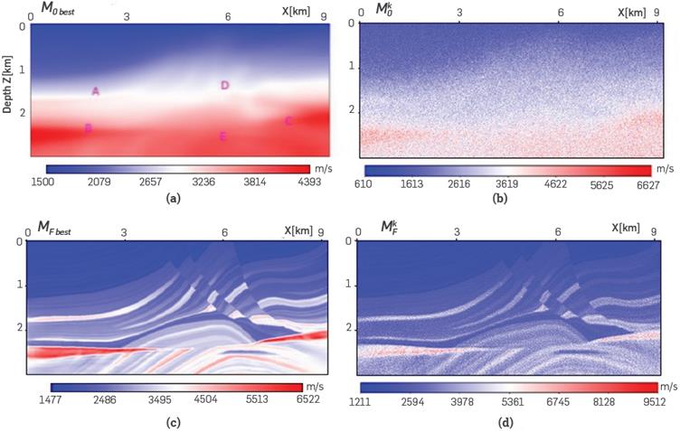
Figure 3 (a) The fiducial initial model, M _{0 best} , and its fiducial inverted model, M _{F best} , in (c). A perturbed initial model, M ₀ ^k , for k=56, and its FWI, M _F ^k , are displayed in (b) and (d), respectively. 

The fiducial inverted model M _{F best} , with pixels accomplished by applying FWI to M _{0 best} , is shown in Figure 2c, for the Diffractor model, and in Figure 3c, for Marmousi. The symbol M _F ^k is used for the kth model of the cube, that contains nm inverted models obtained by applying FWI to the kth perturbed model in M ₀ ^k , as shown in Figures 2d and 3d, for Diffractor and Marmousi models, respectively. The set of final outputs, is used for quantifying the uncertainty of the velocity profiles.

The statistical experiment was carried out in the same way for the two models: Diffractor and Marmousi. The cube of nm initial models was inverted through FWI, by using synthetic data obtained from propagations in the M _real , and by using the frequencies, (ω ₁ , ω ₂ , ω ₃ , ω ₄ ), in the multiscale procedure for all models.

Figure 2e shows the distribution of velocities of the initial model cube for the pixel (70,20). It was confirmed that the distribution of every pixel, for both models, satisfied a quasi-normal distribution. Based on the quasi-normal distribution of the velocities and, based on the central limit theorem (which requires nm ~ 30), we are confident that nm=100 starting models represents a great sample for our experiment.

USUAL ANALYSIS OF THE UNCERTAINTY

The uncertainties of the FWI were analyzed using the nm final inverted models, taking the jth multivariate random variable as the vector mj = (c _j ¹ ,…,c _j ^nm ). Thus, the final cube, M _F , of inverted models can be considered a tensor M _F =(m ₁ ,...,m _NP ).

The traditional quantification of uncertainties is made through the estimation of a map, σ(z,x), of the standard deviations with a priori mean for each pixel as the square root of the variance

DENSITY OF CORRELATION MAPS

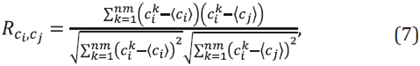
The σ(z,x) map is a method used to quantify uncertainties. However it uses data only from the diagonal elements of the covariance matrix. Off diagonal terms of the covariance matrix may differ from zero, and if that is the case, important information can be extracted on the correlation induced between different elements of the velocity model. In this work, we estimated the covariance matrix as

Where each entry is an estimate of the relation of the velocity values of the two pixels c _i and c _j . It should be noted that this is a general estimation. No assumption about the nature of the underlying distribution of the uncertainty is made, and it is not a diagonal matrix. Indeed, it is possible that, without focusing on possible pathological cases, if an entry cov[c _i , c _j ] has a large absolute value, then the uncertainty is increased, as the distances (c _i ^k -⟨c _i ⟩) and (c _j ^k -⟨c _j ⟩) are large. Similarly, if it has a small absolute value, the uncertainty is expected to decrease.

Thus, the cov[c _i , c _j ] matrix contains relevant information about the uncertainties that is not included in the analysis of the standard deviation map that only takes into account the self-correlation. To simplify the analysis, we will work with the correlation matrix R, which we estimate as

R matrix carries the same information as covariance matrix, but this normalized form helps to understand, among other aspects: (a) How the wave velocities are correlated within a model. (b) The meaning of the correlation between velocities. (c) The relationships that exist between the correlation of the pixels and the uncertainties of the velocities associated with those pixels. The R and covariance matrix contains data that is not usually analyzed in the description of the uncertainties in FWI. Maybe, a reason to keep it out of the discussion is related to its size. Since for a set of NP random variables, R is a NP ² sized matrix, the size of such data set becomes a challenge. For example, for the simple Marmousi model used in this work implies the requirement of 153Gb of memory in double precision, which is quite large for such a small model. Hence, a reliable estimate of uncertainties analysis for FWI turns to be expensive. In comparison, the methods that use the resolution matrix, opt for the Hessian, which dimension is NP, and it requires less computational resources, although it contains less information. If we want to know more about the uncertainties in FWI, we must necessarily use more computational resources and all the information contained in R.

We compute the R matrix for both, the Diffractor and the Marmousi models. We visualize R as a collection of NP sub-matrices, each one of size NP. For example, the correlation matrix R _c7580cj , ∀ _j = 1,…,NP, will symbolize the sub-matrix of correlation of the pixel c ₇₅₈₀ with the rest NP pixels in the model. Figure 4a shows the matrix R _c7580 .

The mth sub-matrix, R. , is a map with ordered elements ( R _ci , _ci ,…, R _ci , _cNP ). The element R _{ci , ck +nz*l} symbolizes the correlation of the pixel c_i with the pixel c _k+nz*l ; where every value was computed using equation (7). Using this nomenclature, the k/-th element of the matrix R . , will be given by R _{ci , ck +nz*l} . Figure 4a shows the correlation map of submatrix R _{c 7580} . The continuous blue band at the top of the map corresponds to the first 40m that were not inverted. The red point inside the circles shows that the pixel is completely self-correlated. In general, visualizing and extracting information from matrix R is not trivial because of its large size. On the other hand, one might be interested in to see how strong is the correlation between a pixel and its close neighborhood. It is not actually expected to see any correlation between pixels that are too far away from each other. Therefore, to look for correlations between pixels, and in order to simplify the analysis of the information in the full matrix R, we are proposing a method intended to accomplish these goals.

We propose to associate only one real number D _i ., to each R _i . matrix. D _i will be named "The Density of Correlation" of the pixel c _i . Let (pΔz,qΔx) be the physical position of the pixel c _i , see Figure 4a.

D _i is computed by averaging all values of the correlation inside a ring of width Δ=r _n+1 -r _n , for n = 0,1,... ; and center at (pΔz,qΔx). Such an average is divided by the area of the ring. In this manner, each ring is labeled through an integer n: n = 0 accounts for a circle containing the first neighbors only, n = 1 label the first ring, and so on.

For example, the density of correlation of each pixel with its first neighbors, where the ring becomes a simple circle with r₀=0 and r ₁=min (Δz,Δx), is estimated without including the self-correlation value, as

such that |(pΔz,qΔx)-(kΔz,lΔx)| ≤ r ₁, where N is the total number of correlation values inside the circle of radius r ₁ .

It is expected, from the physical point of view, that the largest correlation of the pixel c _i ., will be associated to its first neighbors, as the arriving wave to the pixel comes directly from such first neighbors. This physical fact was computationally explored, by analyzing the behavior of D _i as a function of n, which is shown in Figure 4b. Let A _n = π (r _n ² -r ² _n-1 ) be the area of the n-th ring, then the quantity |A _n D _i (n)| accounts for the absolute value of the average of the correlation values in the n-th ring. Figure 4b presents |A _n D _i (n)| for the first 20 radial bins for c _i = c ₃₇₅₂₅ in the Marmousi model. It should be noted that the intensity of the correlation averaged for each ring decreases rapidly for the first 5 rings, regardless on the normalization effect of by the geometric factor A_n in equation (8). The same behavior was evidenced by all pixels in both velocity profiles. Thus, we confirmed that correlation is a local effect and the density of correlation D _i can be calculated for the first neighbors without compromising much data. Thus, by using D _i we have reduced the data of sub-matrix R _i into a number D _i representing the density of correlation of pixel c _i with its neighbors. Thus, the full data of the R matrix is reduced from a matrix of size NP ² to a single matrix of size NP. The association of a number D.with each R _i matrix, results in the concept of Density of Correlations Map D _n (z,x), for a ring with a maximum radius r_n, defined by the collection D _n (z,x)={D ₁ ,...,D _NP } and with units m ^-2 . Similarly, by using an identical analysis, we can define the Density of Covariance Maps Cov _n (z,x), for which the equation (6) is used. The analysis presented in this work were built for the first neighbors, n = 0, and then we will simplify the notation as D ₀ (z,x)=D (z,x) and Cov ₀ (z,x) = Cov(z,x).

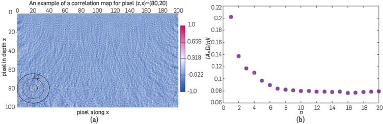
Figure 4 (a) Rings used to compute D _i by averaging all values of the correlation inside a ring of width Δ, with center in the physical position of the pixel c _i , such average divided by the area of the ring, (b) | A _n D _i (n) | as a function of distance, for the first 20 rings. The intensity of | A _n D _i (n) | decreases rapidly. The same behavior was verified for all pixels in both velocity profiles. 

MEAN VALUES MAP 〈M _F (z, x)〉: DIFFRACTOR MODEL

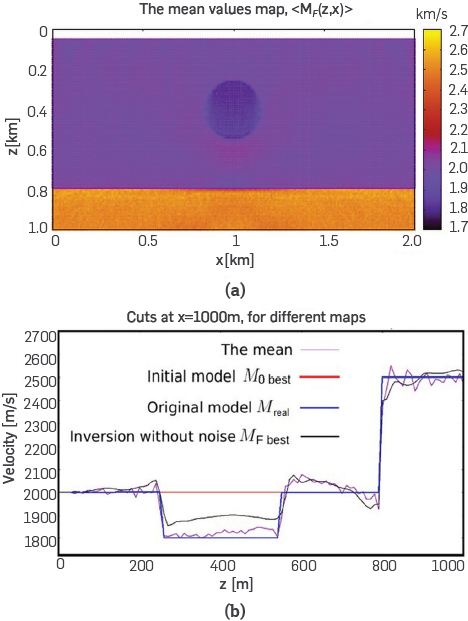
The Diffractor model has the parameters nz = 101, nx = 201, Δz=Δx=10m, and NP =20301. The dimensions are 1km in depth, and 2km in x. In order to do every FWI, ns = 11 sources were disposed at z _s = 40m, and x_si. = (1000 ± i*200)m, where i=0,1,2,...,5. A receiver is located at each grid point along the x axis, then nr = 200; and z=0m. The frequencies (ω₁, ω₂, ω₃, ω₄)=(10,20,30,50)Hz were used in the multiscale, with 5 iterations for each frequency. This model consists on a first layer, z ∈ [0,750]m, with a wave velocity of 2000m/s and a second layer, z ∈ (750,1000]m, with a velocity of 2500m/s. The first layer contains a circular object, labeled as Diffractor, with a radius of 150m, and centered at ( z _c , x _c )=(400,1000)m. The mean values map 〈M _F (z, x)〉, which was built using equation (4), is shown in Figure 5a. Figure 5b shows several vertical cuts at x = 1000m, a cut for 〈M _F (z, x)〉, a cut for the initial profile M _{0 best} , a cut for the real profile M _real and a cut for the fiducial inverted profile M _{F best} . Although this figure is presented only for x=1000m, the features discussed hold for every x, as we verified cuts for x=10m,20m,…,1990m.

Note that the mean velocity (violet line) is closer to the real (blue Line) than the inverted fiducial model (black line). Just inside the circular object and its surroundings, the difference between M _{F best} and M _real has the highest value. As a general observation, such difference increases in the neighborhood of each interface, i.e., the interfaces are sources of uncertainty.

When the waves reach the zone z > 750m, they have crossed three boundaries: z = 250m, z ~ 550m, and z ~ 750m; and we note that the discrepancy between the different FWI shown in Figure 5b does not grow uniformly while depth increases. Thus, such discrepancy is low for Om < z < 250m, later the discrepancy increases inside the circular diffractor, and in the subsequent meters 250m < z < 750m; and for z > 750m, the discrepancy decreases. However, such decrease does not mean a decrease of the uncertainty with depth, as Figure 5b does not show a standard deviation map. Figure 5b is merely a comparison of a FWI cut. In deeper positions, there is Less illumination, and the physical consequences are shown as an increase of the uncertainty, see Figure 6b.

Figure 5 (a) The mean values map. (b) Comparison between the mean values map 〈M _F (z, x)〉, the initial profile M _{0 best}, the exact profile M _real, and the best inverted profile M _{F best}, for x=1000m.  

UNCERTAINTIES ON VELOCITIES: DIFFRACTOR MODEL

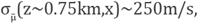
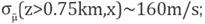
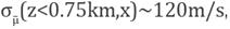
Figure 6a, measured in pixels, shows how the standard deviation ncreases with depth, having a jump just around z ~ 0.75 fcm~80 pixels. The zone z ~ 0.75km, σ_µ ^- (z,x) shows the greatest contrast. This fact is a natural consequence of the little illumination reaching the bottom of the velocity profile. Just in the interface of the two Layers, the uncertainty increases. This fact is in agreement with Figure 5b, where we argued that the discontinuities are a source of uncertainty.

Figure 6b shows vertical cuts in the standard deviation map at different positions along the model. As it can be observed in the curves, there is a different behavior of the variation of uncertainty away from the circular diffractor than when it is close. Violet and black curves show that the standard deviations, close to the boundaries of the model, are larger than the standard deviations near the center, which are shown with blue, red and green curves. This fact is quite different inside the circular diffractor. Figure 6b clearly shows a global, systematic and almost linear increase of uncertainty with depth. An interesting fact related to FWI is that after a reflector (an interface), the variance decreases locally, i.e., the map and however i.e., such decreasing in merely local: always grows globally.

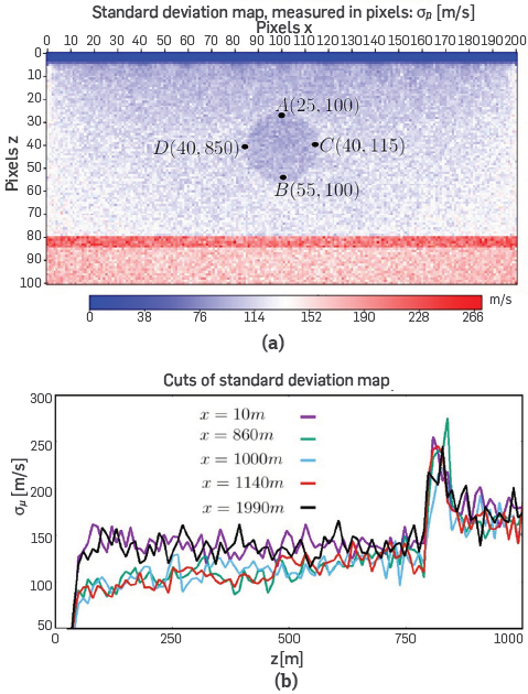
Figure 6 (a) The standard deviation map, with previous mean µ^-, σ_μ̅ (z, x) of inverted models {M _F ⁱ }, resulting from FWI process, (b) Several cuts of the σ_μ̅, showing the increasing of the standard deviation with depth. 

MEAN VALUES MAP 〈 M _F (z, x) 〉: MARMOUSI MODEL

All data about the Marmousi model used in this paper is available in the Madagascar repository ^[24]. This model lies under water approximately to 32m. It has 9.2km along x-axis, and 2.992km along z-axis. It contains 158 horizontal layers and its extreme velocities are c_min=1500m/s and c_max=5500m/s. The parameters used in this experiment were nm = 100, nz = 375, nx = 369, Δx=0.025km, Δz=0.008fcm. A receiver is located at each point along the x-axis, therefore, n_r=369; and z _r =0m. The number of sources is n_s =62, with z_s =40m, and x _si = i*150m, where i = 0,1,2,…,61. The frequencies used in the multiscale were (ω₁, ω₂, ω₃, ω₄)=(10,20,30)Hz. In the inversion, 30 iterations per frequency were required, i.e., six times more than the number of iterations used for the Diffractor model. Thus, in order to reach M _{F best} the total time computation increases about 24 times as compared with the Diffractor model.

The mean values map 〈M _F (z, x)〉, for the Marmousi model is presented in Figure 7, as well as the lateral changes in velocity belonging to M _{F best} . Note that the complex zones, as those highlighted in white, circles and box, are recovered for the FWI.

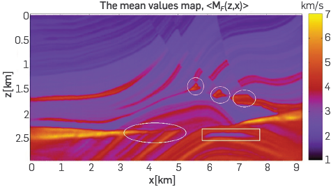
Figure 7 The mean values map, accomplished by doing FWI to the initial cube M ₀. Complex details of the model, as those highlighted in white, are present in both, M _{0 best} and 〈M _F (z, x)〉.  

Figures 8a and 8b show vertical cuts at x=6.5km and horizontal cuts at z=2km _l comparing the mean, the exact, the initial fiducial model, and the inverted fiducial model. In both figures the discrepancies between the results of the inversion are minor. Although the mean shows larger discrepancies as compared with the exact model than the M _{F best} , a better quantification of such discrepancies may be revised in the standard deviation map, in order to check the places where the inversion introduces more uncertainty.

UNCERTAINTIES ON VELOCITIES: MARMOUSI MODEL

Figure 9a shows the standard deviation map. The zones with greater uncertainty are those with strong lateral variations in the velocity profile, for 2km <z< 2.5km.Figure 9b shows the maximum uncertainty around 2.5km/s, for the cut z=2.330km. The exact velocity in this zone, with strong lateral changes, is 5.5km/s, and Figure 9c implies that the error for this zone is close to 45.45%, which is undesirable. However, only two zones show this behavior and the rest of the map shows a standard deviation of ~0.5km/s, which is acceptable.

Figure 8 Comparison between the mean, the exact, the initial, and the inversion without noise, named M _{F best.}  

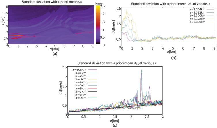
Figure 9 (a) The standard deviation σ_μ̅(z, x), of the inverted cube M _F, resulting from the FWI to the cube M ₀. (b) Several cuts for the zones with greater uncertainties, which is caused by the strong lateral gradients. Not considering the large peaks at 2km < z < 2.5 km, the functional shape σ_μ̅(z, x), is, on average, a line whose slope is around 2.34s^-1; as is shown in (c). 

Figure 9c shows that the functional shape of σ_μ̅(z, x) has a global Linear growth of uncertainty. The slope for the cuts is close to 2.34s^-1. Considering the detail of the fluctuations shown in Figure 9c, it is evident that the uncertainty has strong fluctuations in the region 2km < z < 2.5km, where there are strong discontinuities in the profile as observed in Figure 9a.

Going back to the same behavior observed in the case of the Diffractor, we notice that when there are strong discontinuities in the medium, uncertainty grows locally in the region of the discontinuity. After seeing this effect on the artificial model of the Diffractor, and in this more realistic situation of Marmousi, we suggest that this is an issue to be considered. We suggest that this increased uncertainty may be caused by the behavior of the modeling of waves in such discontinuities, where caustics of waves may appear due to the modeling of interfering waves in these regions. Note that once discontinuities are overcome, in region z > 2.5km, the standard deviation collapses, for all vertical cuts, to the same regular behavior.

ANALYSIS OF DENSITY OF CORRELATION FOR THE DIFFRACTOR MODEL

We now move to the Density of Correlation and Density of Covariance maps. To make sure that the experiment is unbiased, we show in Figures 10a and 10b the absolute value of the density of correlation |D(z,x)| of the initial cubes M₀, for the Diffractor and Marmousi models. From Figures 10a and 10(b), it can be observed that there is neither a preferred direction nor systematic fluctuations in the initial conditions map, which means that the random noise, introduced to each pixel in our experiment, leads to ndependent and uncorrelated initial models even when the M _{0 best} comes from a smoothing of the M _real .

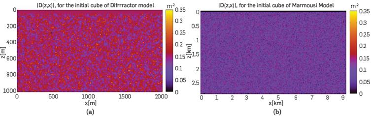
Figure 10 D(x,z) for the initial models. (a) for the Diffractor, and (b) for the Marmousi. The maps show a uniform distribution of the Density of Correlation indicating non-biased initial data. 

Figure 11a shows the absolute value of the Density of Correlation map, and Figure lib shows the square root of the Density of Covariance map. It may be noticed that, although major structural features (as discontinuities) can be observed in both maps, the different normalization enhances diverse characteristics in each. For example, in the map, Figure lib, the discontinuities of circular diffractor and the change of layer than in Figure 11a are clearer, whereas the white rectangle does not contain such change, and the circular diffractor is diffuse. Comparing 11a and lib, it can be observed that in the |D(z,x)| map (see the green squares), it is easier to observe the artifacts (noise in the correlation) on the borders, due to the boundary conditions. Figure 12a shows vertical cuts at different positions at the borders and the center of the profile. Violet and green lines show, in agreement with what is seen in Figure 11a, that there is a low correlation between pixels at the border, |D(z,x)| _max ~ 0.2m ^-2. The correlation in this region, x~10m or x~1000m, decreases as a function of distance from the surface falling down almost to zero at around 600m. We suggest that the behavior of the correlation of pixels close to the borders may be related to the effect of boundary conditions, indicating that they behave partially as a reflector. In the region of the middle of the model (blue line) of Figure 12a, we can see that the density of the correlation is bigger, |D(z,x)| _max ~ 0.5m ^-2., and it systematically decreases with z. This last behavior matches the findings of the analysis of standard deviation maps, where standard deviation increases smoothly with depth.

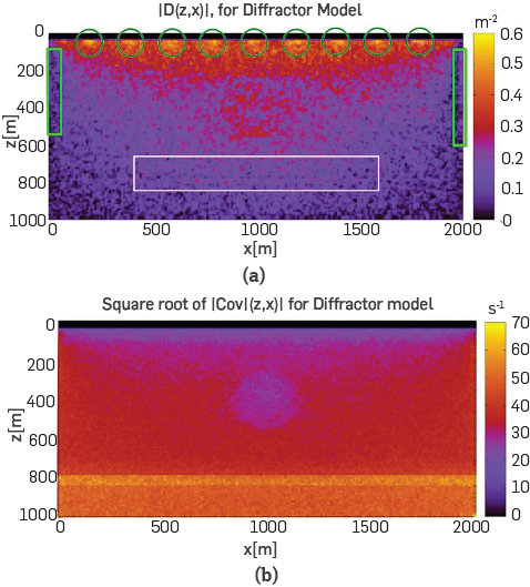
Figure 11 (a) |D(x,z)| for Diffractor model. A decrease of uncertainty in well illuminated zones is evidenced through the increase of the values of Density of Correlation, which are near to the sources in the D(x,z). The white rectangle highlights a limited definition of the interfaces, unlike to a better definition shown in (b), where | is illustrated. 

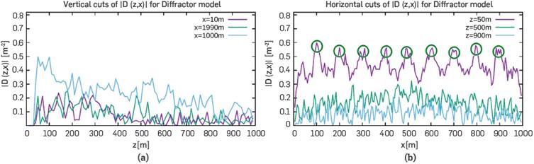
Figure 12 (a) Vertical cuts of |D(x,z)| at different horizontal positions, (b) Horizontal cuts at different depths. The circles show the 9 peaks, corresponding to the sources, showing that the energy sources correlation with the pixels. 

An important feature of the Density Correlation map, |D(z,x)| is the possibility to observe the positions of the sources through the peaks of correlation, which are highlighted with green circles in Figure 11a. Thus, there are peaks in the correlation due to the presence of the sources. Remember that, for the Diffractor model, the 11 sources were disposed at x_s={0,200,400,600,800,...,180 0,2000}m. The effects of the boundaries mask the first and the Last peak, corresponding with x_s=0m and x_s=2000m. Thus, D(z,x) shows that there is a strong correlation between the sources and its neighborhood. Assessing how this correlation affects the quality of the inversion is out of the scope of this work, but this diagnostic can be used to study the impact of the configuration of seismic sources on the final result of FWI. If we consider that large correlations are associated to small uncertainties (small cross-deviations from the mean value) it also implies that modeling the source is a key ingredient in FWI. The fact that the correlation can be other than zero in certain zones suggests the existence of physical data correlating the elastic properties of the pixels in the subsurface model. Such physical data comes from the seismic data, both d _o and d _c . These two data vectors contain relevant information on physical relations between different pairs of pixels inside the model and, therefore, D(z,x) is large when there is a high correlation of those vectors. Obviously, close to the surface there is physical data available that correlates pixel values. For example, the correlation ϑ of the observed and modeled data has been described by ^[23] as:

The cuts shown in Figure 12b agree with equation (9), having peaks around the sources, where the observed and synthetic data share the greatest amount of available information. Thus, the procedure to analyze the correlation matrix through the Correlation Density maps reproduce natural facts as the correlation between synthetic and observed data. The D(z,x) maps provide information on uncertainties around the sources that is not evident in the other two maps: The Standard Deviation σ(z,x) or The Density of Covariance Cov(z,x).

So far we have stated that the correlation between two different points suggests that their uncertainties are related, but such relation (the functional shape) is unknown and, therefore, an uncertainty analysis of the three maps, σ(z,x), Cov(z,x), and D(z,x), may be used.

DENSITY CORRELATION ANALYSIS FOR THE MARMOUSI MODEL

The Cov(z, x) and D(z,x) maps were computed for the Marmousi model, which show similar results to those discussed for the Diffractor. In the Cov(z, x), the decrease of uncertainties derived from the effects of boundaries was verified However, due to the complexity of this model, the range of values of this map oscillates in the range [0,300² ) m²/s²; such an interval is very large and, therefore, the visualization of the information is somewhat unclear, To better visualize this map, we include its square root, , in Figure 13a. Using this scaling, the contrasts are larger and it is possible to observe that, besides the boundaries, in the zones with high lateral gradients of velocity, the covariance (the uncertainties) increases. Figure 13a reveals that there are several physical or geometric features, other than illumination, which increase the uncertainties. Figure 13a shows zones enclosed in white squares and rectangles, and also zones pointed at with white arrows. The two smaller arrows point towards zones with Cov(z, x)~ 200m/s, with depths z ~ 1.5/cm, while the smallest rectangle, with Cov(z, x) < 100m/s, is deeper z ~ 1.9km. The same phenomenon exists for the larger white arrow, which points to the highest wedge (z ~ 2.5km) associated to ~250m/s, while the white squares point to zones (z ~2.7km) associated to ~130m/s. Beyond the illumination, the physical (geometrical) properties of the model and the properties of the ingredients of the FWI engine produce quantifiable changes in the uncertainties. Such ingredients were described in section 2. The map and its properties are very similar to the mean value map 〈M _F (z, x)〉 see Figure 7. This fact comes stems from the contrast of velocity magnitudes, which are reflected in the map.

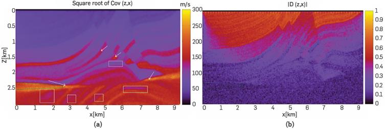
Figure 13 (a) Cov(z,x) map of Marmousi model. There are several physical or geometric features, other than illumination, which increase uncertainties, (b) The |D(z,x)| map containing 61 peaks, with correlation values close to 1, and corresponding with the 

The mathematical standard deviation concept is close to that of the covariance map square root; therefore, the map is practically identical to the σ_μ(z,x) map, see Figure 9a. Such similarities enable relying on the algorithm and the method used to compute Cov(z, x) and D(z,x). An important fact to note, which is valid for all the cases studied herein, is that the Density of Covariance (coming from all elements of the matrix cov[c_i,,c_j]] differ from zero almost everywhere. This means that not all information of uncertainty in FWI is in the σ_μ(z,x) map (which comes from diagonal of cov[c_i,,c_j]]), since σ_μ contains numerous values close to zero, see Figure 9a.

Figure 13b shows the absolute value |D(z,x)| map. Once again, it can be noted that for those zones with large uncertainties (large Cov(z, x)), the correlation density values are close to zero. The growth of the uncertainties coming from different causes with depth, is verified again. Zones such as those enclosed by green Lines reinforce the interpretation of section 3.3: zones of Cov(z, x), where the covariance increases entails zones of D(z,x), where the uncertainties grow. From a general perspective, the |D(z,x)| map reproduces the main features found for its analogous in the Diffractor. The uncertainties grow with depth and with proximity to the boundaries. Also, Figure 13b, contains 61 peaks with correlation values close to 1, and corresponding with the positions of the sources (z_s,x_si = (0.004,/*0.15)km, with i=0,1,...,61. As it was already highlighted, the correlation density map can determine the correlation between the sources and the model,