English (pdf)
 Article in xml format
 Article references
 Send this article by e-mail
 Cited by SciELO
  Cited by Google
  Similars in
SciELO
Similars in
SciELO  Similars in Google
 Permalink
1. INTRODUCTION
Polymers increase water viscosity and reduce the water-oil mobility ratio. Polymers generate a uniform flow and prevent a phenomenon called "fingering," which leaves the oil behind the water solution 1. HPAM (Partially hydrolyzed polyacrylamide) present high solubility on the water; however, the viscosity of the polymers is affected in high temperatures and salinity 2)-(4 conditions. HPAM polymer's chain degrades by the high shear experienced, reducing the viscosity and decreasing the efficiency of the oil recovery process 5),(6.
Polymer flooding has been evaluated at a field scale for more than five decades, and it is becoming an increasingly more interesting technology within the oil and gas community 7. In any oil field, there are devices in surface facilities for polymer flooding of different sizes; therefore, it is possible to find a change in diameter between the oil field facilities and the injectivity well. Choke valves, static mixers, injection pumps, distribution lines, and other accessories could generate more than 50 percent viscosity degradation 8),(9. Usually, viscosity loss of 20% or less is common in this type of project 10.
Experimental studies of mechanical degradation focus on measuring viscosity changes, flow velocity, and shear rates of the polymer solution since the beginning to the end of the tubings, capillaries, and porous media 11)-(14. However, it is essential to obtain data on fluid dynamics in turbulent flow conditions, which is challenging to obtain in a laboratory. Hence, it is necessary to use numerical simulation to assess the behavior of polymers flowing between different diameter sizes.
Many authors report studies on numerical simulation related to the viscoelastic fluid effect in contraction and expansion geometries. Moreover, many of the numerical simulations focus on porous media 15)-(17 or the study of the contraction and expansion flow with low Reynold numbers 18)-(21.
In this research, the polymer solution is rheologically characterized through viscosity and shear rate curves to set the mathematical model that fits better with the experimental data. Then, a viscosity degradation model was built using capillary tube tests; the model compares the viscosity degradation with the shear rate. Finally, with the viscosity model and viscosity degradation model used in Ansys Fluent 22, the results were validated based on laboratory data of polymer solutions flowing through restrictions.
2. THEORETICAL FRAMEWORK
MATHEMATICAL MODELING
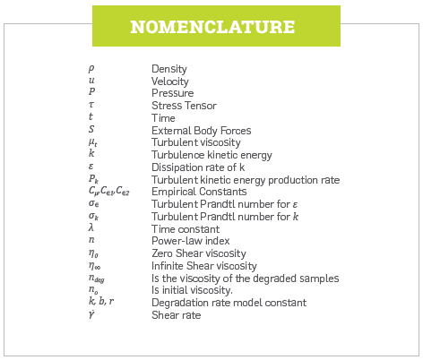
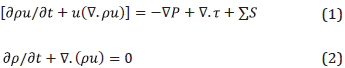
Computer Fluid Dynamics is a numerical tool based on the solution of the transport equations that describe the flow of fluids in a controlled volume. Discretization methods adjust the partial differential equations into a group of algebraic equations, which enable the solution using numerical methods. It is necessary to divide the physical domain into volume elements, which is referred to as computational mesh, where those elements solve the transport equations (equations of balance). The software solved the partial differential equation of momentum (Equation 1) and continuity (Equation 2) representing the fluid mechanics, where ρ density, u velocity, t time, P pressure, τ stress tensor, and S external body forces.
TURBULENCE MODEL
Polymer flooding takes place in turbulence conditions on surface facilities and some accessories; for example, Reynolds numbers are over 3,000 when the polymer runs through valves of diameters ranging between 2 and 4 mm. To describe the turbulent flow, the k-epsilon model was used in simulations; this model considers a turbulent viscosity (different from the molecular viscosity), which depends on a regime flow and depends on the fluid's position, velocity, and properties. Therefore, the kinetic turbulence (k) and dissipation viscosity rate (ε) shown in transport equations (4 and 5) are related to turbulence viscosity through (3).
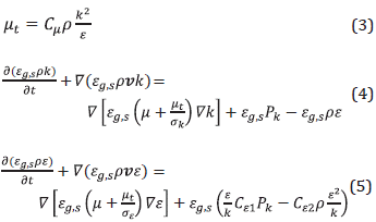
where P k is the turbulent production of the viscous forces, and C^Ce1,Ce2,ae,ak are empirical constants.
RHEOLOGICAL MODEL
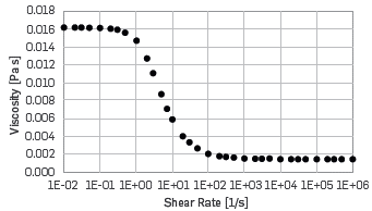
The HPAM is no Newtonian fluid, as viscosity is a function of the shear rate. Most of the HPAM have a pseudoplastic behavior, which explains the viscosity decrease as the shear rate increases 2, as shown in Figure 1.
Equation 7 presents the Carreu model, which sets the pseudoplastic behavior and correlates the stress tensor (Equation 6), represented in the second term of Equation 1 with the viscosity of the polymer analyzed.
Where τ is the stress tensor, y is the shear rate tensor. Parameters λ and η are empirical constants of HPAM, white η 0 and η„ are the Limits of Lower and higher shear rate viscosity.
MECHANICAL DEGRADATION
The energy required for mechanical shear degradation is obtained from the mechanical energy applied to the shearing process. The bond rupture may occur if the energy introduced into a bond exceeds the binding energy 24. The percent Mechanical degradation (% DR) was calculated using the following equation:

Where n deg is the viscosity of the degraded samples, and n„ is the initial viscosity
3. EXPERIMENTAL DEVELOPMENT
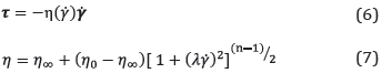
As regards experimental data, this research assesses two different HPAM polymer concentrations prepared in distilled water. Then, the polymer fills the cylinder shown in Figure 2, and flows through to the capillary and another two geometries connected at the bottom of the cylinder.
The polymer flows through geometries because of the pressure drawdown generated with the nitrogen line connected to the top of the cylinder. The viscosity of the polymer solution, as shown by Equation 8, is measured before and after the mechanical degradation
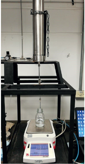
The proposed methodology (Figure 3) in this paper starts with the polymer solution characterization, building a viscosity vs. shear rate curve. Next, degradation model data was developed using capillary devices. When degradation and rhéologie models were set with Matlab codes, the next step consisted in creating the overall study geometry and establishing simulation conditions similar to those of the real experiments. Subsequently, once the independent mesh is obtained, this methodology figures out the most significant degradation on different geometries. For that purpose, the method analyzes the velocity profile to locate the specific plane where the acceleration and strain rate is greater. Finally, combining this variation of velocity and strain rate with the most significant change of the degradation rate, a transversal plane is created at the exact point to calculate the area-weighted average degradation rate in this zone.
RHEOLOGICAL DATA
Expérimentât data of HPAM polymer solution of different concentration were measured in an Anthon Paar MCR 702 rheometer, using concentric cylinders at 303.15 kelvin (30°C).
DEGRADATION MODEL
Polymeric solutions show mechanical degradation in the presence of high-shear rates due to shearstress in the flow; measuring these mechanical degradations is essential for the viability of the project. In this research, we implemented the recommended practices for assessing Polymers used in Enhanced Oil Recovery Operations (API RP 63) 25 to obtain different degradation rates at different shear rates. This practice uses a capillary shear device given In Figure 2, where the polymeric solution flows from the cylinder to a capillary of a determined diameter.
MODELS SETTING
The mechanical degradation (%DR) is related to different shear rates; a logical model of population growth correlates mechanical degradation and shear rate using Equation 9

Where k,b,r are the model's parameters, and γ is the shear rate. These parameters are determined experimentally.
To determine the empirical parameters of the mechanical degradation, the numerical algorithm of the least-squares implemented in the software MATLAB R2017® 26 use experimental data. The algorithm finds the model coefficients that satisfy Equation 10 with entry data (xdata,ydata):

Where, (f(x,xdata,) is the evaluated matrix of the setting function with the experimental data, Equation 11, where the vector* has the same parameters of the model.
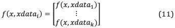
After obtaining the parameters, the User-Defined Function (UDF) ntroduces the empiric and viscosity models to the CFD to estimate the mechanical degradation values (%DR). Figure 4 shows the approximation obtained from laboratory data using the logistic model of growth of the degradation by capillary shear and non-linear regression for the viscosity model of Carreu, respectively
As shown In Figure 4d, the percentage error is less than 20 in all cases. As regards 4c, only one experiment has a value greater than 30%. This percentage demonstrates that the model predicts and represents, in most cases, the degradation and viscosity with slight differences. Furthermore, some cases with a percentage error greaterthan 10% could explain the differences between simulation data and experimental data. Also, experimental measures include human and laboratory devices error.
CONFIGURATION OF THE SIMULATION MODEL
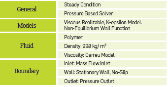
The configuration of the rheological and the physics of the fluid properties, as well as the operating and boundary conditions, and numerical aspects Inherent to the methods used, are necessary for the numerical solutions of the mathematical models that describe the transport phenomena inside the geometries. The accuracy of results depends on the configuration In the CFD simulation.
After defining the rheological properties, the boundary conditions, and the initial conditions of the simulation model must be identified. Table 1 shows the simulation conditions. The simulation considers an Isothermal system and incompressible flow. The wall boundary condition finds the non-slip condition, providing an effect of the boundary layer on the wall. Moreover, the non-equilibrium wall function Is suggested in complex flows where the mean flow and turbulence are subject to pressure gradients and rapid changes. In such flows, improvements can be obtained, particularly In the prediction of wall shear 27,
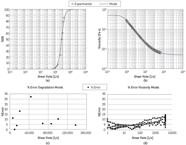
Figure 4 Setting Models, (a) Degradation (b) Viscosity. Percentage error, (c) Degradation (d) Viscosity
Model parameters depend on several factors such as concentration solvent composition, type of polymer, and test temperature. All these factors are specific to the conditions evaluated; hence, it Is necessary to calculate the new parameters for each polymeric solution.
4. RESULTS
CAPILLARY GEOMETRY
Simulation results and experimental results are compared for the narrow cylinder to determine if the degradation behavior on CFD results is close to the empirical data. Figure 5a shows the cylinder with a capillary at the top of the 0.0716 mm (1/8 inch) device.
To discretize the volume of the CAD geometry, Figure 5b shows how the capillary device is meshed. Figure 5c shows that at the center, tetrahedrons are used. While near the wall, the spatial discretization is five layers of hexahedrons with a quadrilateral base.
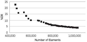
Mesh Independence for the numerical solution is essential; in this case, after 800,000 elements, the difference between the degradation rate is less than 0.05%. The aspect ratio is one of the most critical criteria with respect to mesh quality. In this simulation, the aspect ratio was 10.47, which means a satisfactory quality of spatial discretization. Figure 6 shows the results of mesh independence.
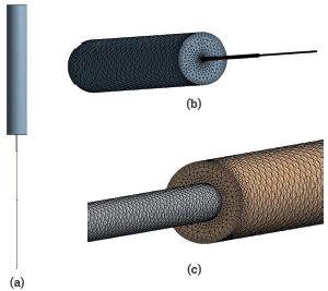
Figure 5 (a)Capillary shear devices built for simulations, (b) Spatial discretization of the Capillary Cylinder created for simulations, (c) Spatial discretization of the Capillary Cylinder close to the capillary.
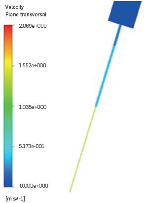
As an initial step, we created a transversal plane to locate the region with the most significant acceleration. This work analyzed all geometry constraints. Figure 7 shows the results for a pressure case of 206.843 kPa (30 psi), where there was an enormous change in the velocity profile in the 0.0716 mm (1/8 inch) capillary, reaching velocities of 2.069 m/s.
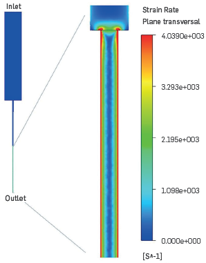
The strain rate depends on velocity changes, as shown in Equation 10. Therefore, high velocity gradients generate pronounced shears nside the geometry.

An important feature is finding the amount of shear in the regulation section on the geometries considering that a high shear rate means high mechanical degradation. Figure 8 shows the shear profile again for the 206.843 kPa (30 psi) case. The most significant value of 4.39xl03 s4 is on the region (last section of the geometry), where the geometries undergo the more critical abrupt changes in the fluid flow.
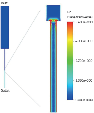
Finally, the degradation rate profile reaches the highest value on the final restriction as predicted by velocity and strain rates. Figure 9 shows the most noticeable degradation close to the wall for the 448.155 kPa (65 psi) case due to the profile of velocity changes in polymers close to the wall is more prominent than in Newtonian fluids 28.
By creating a transversal plane at the top and bottom of the capillary, as shown in Figure 10, we compare the experimental results with the simulation results. The methodology considers the highest area average degradation rate in all the geometry because polymer chains could not recover their structure, and it is impossible to regain their viscosity. Figure 10 corresponds to the 448.155 kPa (65 psi) case, and 1,000 ppm of polymer concentration, where the highest degradation rate is 5,4%, and the experimental degradation rate is 4.7%.
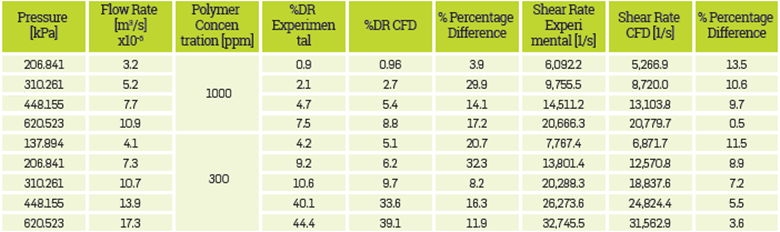
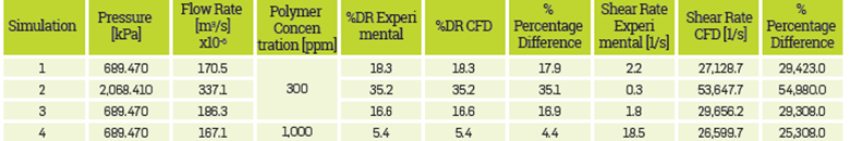
The concentration and pressure conditions were 300 ppm and 1,000 ppm; 137.894 (20 psi), 206.841 (30 psi), 310.261 (45 psi), 448,155 (65 psi) and 620.523 kPa (90 psi). Table 2 compares the degradation rate and shear rate results in the laboratory with the CFD simulations and presents the percentual error, where 6 of the nine data sets show a deviation below 20%. Regarding the shear rate comparison, all data sets show a percentual deviation below 14%.

GEOMETRY A
The second step in this research is to investigate if the degradation model could be applied to other restrictions and represent the phenomena. Hence, geometry A consists of a constraint in the middle of two tubes. This restriction regulates the flow of the polymer before the reservoir injection. Figure 11a represents the CAD geometry in this case.
Figure lib shows geometry meshed using tetrahedrons at the center, and five hexahedrons layers at the wall boundary. The purpose of the refinements at the wall boundary is to properly characterize the turbulence flow of the polymer in this new geometry.
Figure 12 illustrates the results of mesh independence in Geometry A; it reaches the uniform behavior of the degradation rate after 1,500,000 elements because the change of the %DR is lower than the curvature of the first 1,000,000 elements.
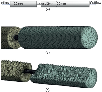
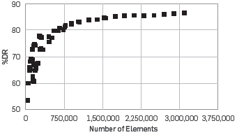
Figure 13a presents the velocity profile at the transverse section of the 2 mm diameter regulation area for the 3,447.35 kPa (500 psi) case. When the diameter changes, the increased velocity reaches 70 m/s.
In Figure 13b, the region where the geometry has abrupt changes presents a high shear rate close to 1.048x10⁵ s_1. As Table 3 demonstrates, the 2 mm and 3,447 kPa (500 psi) case has an area-weighted shear rate of 100,784 s~\ as the highest value of Figure 12b
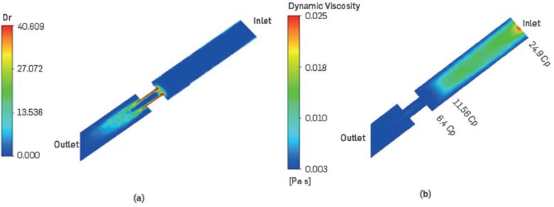
After calculating the shear rate of the fluid, the CFD model correlates these values with the logical model of population growth, determining the degradation rate in each region of the geometry. In this paper, the percentage of the degradation rate was measured in the fluid's bulk subject to mechanical degradation; therefore, Figure 14a illustrates a control region with average degradation. The most significant mechanical degradation was near the part with the highest shear rate, as shown by CFD results for the 2,068.41 kPa (300 psi) pressure drop.
The dynamic viscosity demonstrates in Figure 14b how viscosity decreases near the restriction. At the beginning of the geometry, the viscosity value is the highest (24.9 cP) (0.0249 Pa.s) as the shear rate is close to 0. Viscosity before the 2 mm restriction decreases between 12 cP (0.012 Pa.s) and 5 cP (0.005 Pa.s).
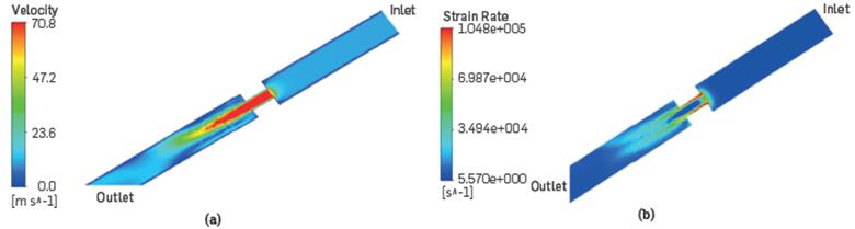
Figure 13 (a) Transversal plane in the Geometry A for the velocity profile, (b) Transversal plane in the Geometry A for the
GEOMETRY Β
As shown in Table 3, results were consistent between the experimental data and the CFD results. The most significant prediction error was about 20% for the degradation rate and 17% for the shear rate. Other results in Table 3 show errors between 3% and 12%.
Geometry Β considers two restrictions of the same diameter, as shown in Figure 15a. At the top of the geometry, the size of the inlet is about 19 mm; then, a small 4 mm tube regulates the polymer flow. Then, another 10 mm expansion appears on the other 4 mm hole. The last 24 mm expansion occurs at the bottom of the geometry.
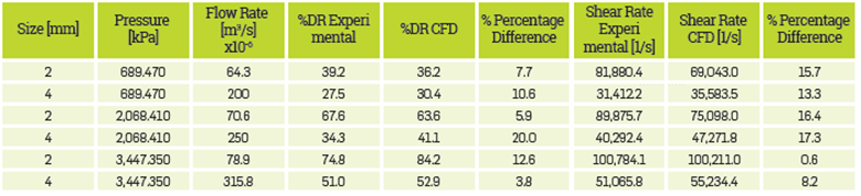
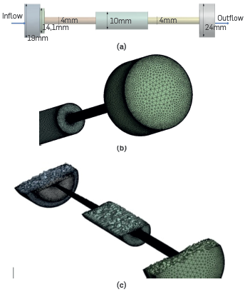
Figure 15 (a) CAD image of the Geometry B. (b) Meshed CAD of the Geometry B. (c) Cut plane in the middle of the geometry
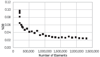
The spatial discretization (Figure 15b), like the previous geometry, Lies in a tetrahedron in the middle of the geometry and hexahedron next to the wall. The latter was useful to characterize the velocity change close to the wall. Geometry Β has inflation and refinement in diameter shift. Figure 16 presents mesh independence when there are over 1,000,000 elements, as the percentage of the degradation rate remains stable. This number of elements in the simulation tests enable performing velocity, strain rate, and degradation contour analyses.
With two restrictions at the beginning and the middle of the geometry, two similar profiles appear in the longitudinal plane. CFD simulations show that the most significant difference of the acceleration for the 2,068.41 kPa (300 psi) pressure drop exists at the start of the minimal size hole, as shown in Figure 17a.
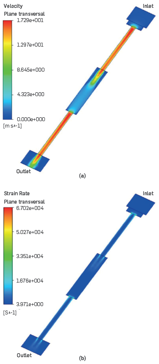
Figure 17 (a) Transversal plane in Geometry Β for the velocity profile, (b) Transversal plane in Geometry Β for the Strain Rate. Two restrictions at the beginning and the middle of Geometry B.
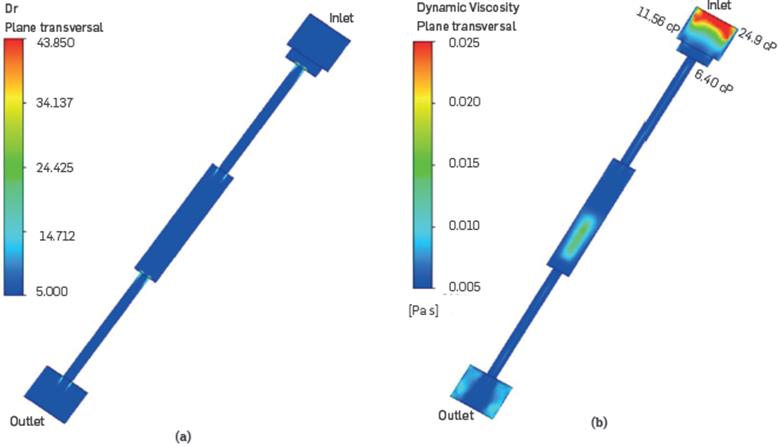
Figure 18 (a) Transversal plane in Geometry Β for the Degradation Rate, (b) Transversal plane in Geometry Β for the Strain Rate.
The strain rate has the same behavior as the velocity profile. Also: the most significant strain rate in Figure 17b for 2,068.41 kPa (300 psi) was on the wall and the top of the restriction hole, where the CFD value is approximately 54,980 s_1. Figure 18a shows the second case of Table 3. The degradation rate matches the velocity and strain rate profiles, where the highest values are in the wall and the restriction. Close to the wall, the greatest degradation on this plane is 43%. However, the average on a transversal plane near the restriction is 35%, which explains the importance of considering the average of a transversal plane and not the higher value. Furthermore: in Figure 18b, the initial viscosity is about 24.9 cP (0.0249 Pa.s) but the viscosity decreases to values of 6.4 cP (0.0064 Pa.s) in the restriction, from 14 mm to 4 mm. In this area, the methodology proposed to calculate the CFD degradation rate is compared with experimental values.
For this geometry, three experimental results correspond to a polymer concentration of 300 ppm and one for 1,000 ppm
5. RESULTS ANALYSIS
This methodology suggests that the most significant degradation occurred at the entrance where the degradation in CFD simulations was evaluated with a transversal plane, as was explained previously Percentual errors of less than 20% in al the three geometries support this theory. However, it is necessary to evaluate more geometries with many contractions and expansions tubes to ensure this phenomenon.
CAPILLARY GEOMETRY
Figure 19 shows that mechanical degradation and shear rate increase with the lower polymer concentration; simulation and experimental results show that a 300 ppm concentration undergoes a higher degradation rate than the 1,000 ppm concentration. This behavior could be explained at a microscopic level, considering the interaction between the Largest chain going throw the capillary restriction. The Large chain in higher concentrations conserve their interaction and do not suffer rupture and dispersion, thus reducing the Lost viscosity
Over 300 kPa (43,5 psi), differences between vaLues of simulation and experimental results increase. Raising pressure drops in the Laboratory means more turbulence. In such an event, predicting the poLymer chain's behavior is more complex, although the difference between experimental and CFD results is less than 10%,
GEOMETRY A
Another relevant result is comparing the degradation rate between 2 and 4 mm (Figure 20). The difference at the same pressure on the degradation rate was about 12 percent, but for 2,068.4 (300 psi) and 3,447.35 kPa (500 psi), the difference increases by over 20 percent. The shear rate is one more aspect that changes with the size restriction. In a 4 mm size at the same pressure, the shear rate is always less than in the 2 mm size. With 3,447. 35 kPa (500 psi) the 2 mm shear rate doubles the 4 mm.
GEOMETRY Β
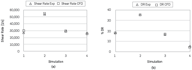
Geometry Β is a particular case, as it has two similar contractions. In CFD simulations, the degradation was assessed in the first restriction achieving the same values as in the experiment. Culter, Zakin, and Patterson 29 proposed in single-pass and multipass laminar capillary flow tests that degradation is independent of tube length Additionally, the main reason to assess the first contraction is that it is more prominent than the second one. The first contraction is from 14 mm to 4 mm, and the second restriction is from 10 to 4 mm.
Figure 21 shows, simulation 2, with the same concentration of simulation 1 and 3, undergoes more significant degradation because of the increasing pressure in these experiments. Furthermore, both figures show that less polymer concentration produces a greater degradation rate, simulation 4 is 5.4%, and simulation 1, with the same pressure but 300 ppm of polymer concentration, is 18.3%,
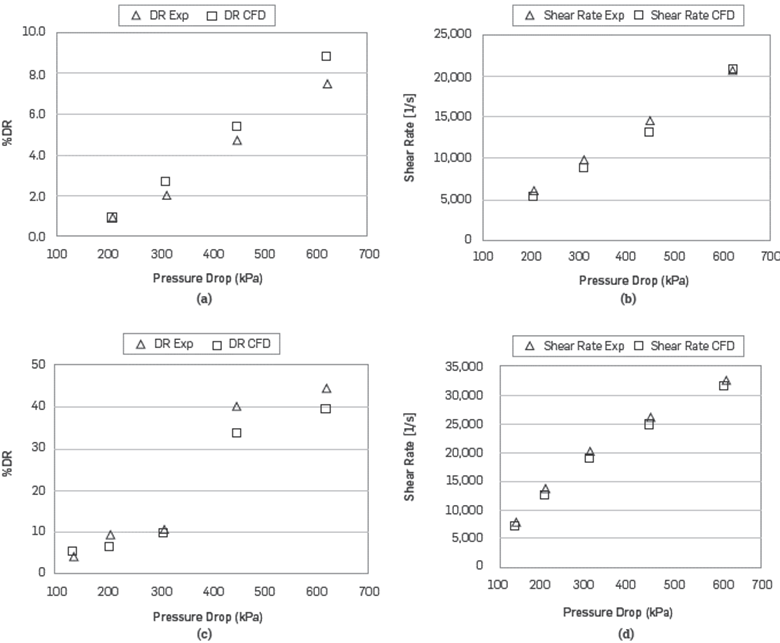
Figure 19 Simulation validation (a) %DR of 1,000 ppm. (b) Shear Rate 1,000 ppm. (c) %DR 300 ppm. (d) Shear Rate 300 ppm.
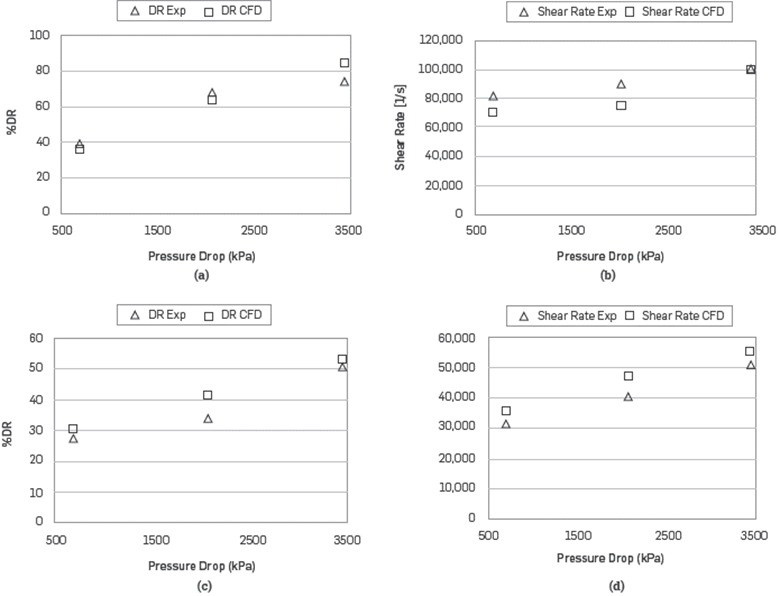
Figure 20 Simulation validation of Geometry A (a) %DR of 2 mm. (b) Shear Rate of 2 mm. (c) %DR of 4 mm.
As demonstrated by the three previous geometries, mechanical degradation increases with a higher flow rate and restriction. These two factors could be represented together with variables like the shear rate. High shear rates are observed in areas with high-velocity gradients, principally because of abrupt flow contractions.
Finally, the methodology proposed to predict the degradation of the polymer in restrictions reaches similar values of real polymer degradations. This methodology helps in the characterization of viscosity losses depending on the type of polymers and facilities geometries. Additionally, with the correct polymer rheology data and degradation model, and a representative CAD geometry for spatial discretization, this methodology could be used in design geometries to reduce the viscosity degradation.
CONCLUSIONS
This methodology, based on CFD simulation, represents a Non-Newtonian fluid using the Carreu model in a turbulent flow, where the mechanical degradation of the polymer correlates with the shear rate of the flow. Comparing three different geometries, CFD simulations and experimental results have an acceptable approximation, where most of the effects show a relative error of less than 20%. Additionally, numerical solutions by the CFD simulations find that the most significant degradation, strain rate, and velocity profiles are on the regions that undergo quick size changes. Consequently, the methodology proposed that the place to validate experimental degradations with simulation results is, in fact, the area with the most significant changes in velocity and shear rate. Lastly, as proven by experimental results and supported by simulation, the degradation of the polymer decreases as the polymer concentration and hole size increase. Larger diameters reduce velocity changes at the outlet, thus creating a lower shear rate. Further, higher polymer concentration produces more durable polymer chains that resist mechanical ruptures.