1. INTRODUCTION

The Location of seismic signals has been commonly performed by methods that require picking of arrivals and correct association of seismic phases among stations; nonetheless, some seismic phenomena generate complex waveforms with no distinguishable phases, thus demanding the use of other methods able to handle both the dynamic and kinematic wave properties. Similarly, wave propagation in real media is complex, and the assumptions commonly made in seismology, such as isotropic and homogeneous layers, become one of several sources of uncertainty. For instance, the location of seismic and microseismic events is typically conducted by ray tracing methods that require correct picking of P- and S- wave onsets, and accurate velocity models that are not always available. The lack of correct velocities may lead to location uncertainty, especially in areas of high structural complexity where the use of ray tracing methods may result in shadow zones and multi-pathing [¹]. Furthermore, combinations of high levels of noise, bandwidth limitations, poor receiver coverage (large azimuthal gaps). and complex source mechanisms, typically encountered during field acquisitions, lead to large location errors from which it is difficult to separate the contribution of each factor [²].

Besides ray tracing algorithms, a more robust family of techniques using full waveform information for hypocenter location has emerged and gained supporters in the last decades. This family is based on the concept of "Back-Propagation" [³], which generally consists of two steps, first, a wavefield U(r,t) generated at either a seismic source or an obstacle (acting as a secondary source) propagates through a medium and is recorded on a set of receivers at different locations r as a function of time t. Then, the receivers are treated as new sources, such that their recordings u_i (r,t) are reversed in time and sent back through the same medium where they interfere constructively or destructively according to the superposition principle. Hence, signals give a maximum constructive interference at the true source location.

In the last decade, most efforts have been focused on developing Backpropagation based location techniques, including Time-Reversal Imaging (TRI) (derived from Reverse Time Migration - RTM in active seismic), which attains the highest accuracy. TRI entails backpropagating time-reversed observations of ground motion through a velocity model; then, assuming an adequate array aperture and an accurate velocity model are used, waves will focus at the true source location. Some relevant studies are: [⁴] where acoustic and elastic propagators are used to locate and characterize 2D passive seismic and tremor-like sources, being able not only to determine location but also radiation patterns; [⁵] modified a TRI algorithm for location of Low Frequency Earthquakes within tremor episodes; [⁶] and [⁷] introduction of new imaging conditions to increase spatial resolution for determination of location and mechanism of microseismic sources in 3D applications. Other authors have reformulated passive source imaging as a Full Waveform Inversion (FWI) problem, using Least-Squares Time-Reversal Imaging (LSTRI) and allowing to jointly invert seismic source information and the velocity model [⁸]. Although TRI is accurate, and commonly used in active seismic applications nowadays, it is computationally expensive as it solves the full wave equation (scalar or vector), requires both accurate velocity models and densely recorded data [⁹], as well as imaging conditions for the forward and back propagated wavefields and, therefore, it is not used in this work.

A simplified form of TRI, known as Back-Projection Imaging (BPI), has evolved as a relatively simple but efficient way to image and characterize active and passive sources. The main difference between BPI and TRI is that amplitude changes due to wave propagation phenomena and polarity changes due to radiation pattern are usually ignored in the former [⁹]. Consequently, BPI produces accurate results while being simple to use and not so expensive computationally, which makes it suitable for sensitivity analysis. Moreover, BPI allows to directly measure the impact of perturbing one parameter on the outcome. These characteristics are desirable since the main purpose of this work is to assess the behavior of a BPI-based location method when some parameters are disturbed.

A significant amount of research has been carried out to understand the impact of several parameters on location of seismic sources; however, most of the publications address the location problem using kinematic methods (travel times only). Some interesting papers are: [²] where common sources of error related to location of microseismic events are presented, concentrating mainly on the effects of acquisition geometry, picking error and incorrect velocity models over the outcome. [¹⁰] This also explains the importance of understanding the effects of noise, velocity and recording geometry on the location of microseismic signals when monitoring reservoirs, hydraulic fracturing and other enhanced oil recovery stimulation processes. Other worth-reading studies are [¹¹] and [¹²]. Sensitivity analysis of TRI-based location algorithms has also been covered in [¹³] where the accuracy of the solution was compared when the number of receivers contributing to the inversion was restricted. [⁶], [¹⁴] and [¹⁵] effects of velocity errors, reduced number of receivers, finite-time source wavelets, and random noise on the solution. Effects of source mechanism, source frequency and station distribution [¹⁶] on location of synthetic volcanic tremor sources. Finally, very limited publications can be found for sensitivity analysis of BPI methods, some of them are [⁹] and [¹⁷] where the influence of array, noise, velocity model and polarity are evaluated. Although some other papers exist on this topic, they are either not easy to find or not conceived as sensitivity analysis but location uncertainty which tackles the problem in a slightly different way. Therefore, there is a need for further research on sensitivity analysis of BPI-based location methods; hence, we attempt herein to make a minor contribution to the geophysical community, especially in our country, by implementing a BPI method that uses waveform information (time and amplitudes) to locate the source of complex signals and allows to clearly notice the effect of individual parameters on the outcome.

2. THEORETICAL FRAME OR STATE OF THE TECHNIQUE

Several seismic source location methods have been developed over the years, seeking to improve the accuracy with which hypocenters can be calculated. According to [¹⁸], most seismic event location methods can be classified into one of the following two main categories: kinematic, which uses arrival times only, and dynamic, which is based on full waveform data. Kinematic methods employ picking of phase arrivals (observed data) and the computation of theoretical arrivals (calculated data) to minimize travel time residuals at each recording station in a given velocity model. Most of these methods belong to one of the following 3 sub-categories: ray tracing [¹⁹], grid-based algorithms [²⁰], and derivative approach derived from Geiger's method [²¹] (implemented on software like Hypo71 [²²], Hypoellipse [²³], and others). Unfortunately, kinematic methods are not suitable for location of complex seismic sources that generate no distinguishable phases in the seismograms or for very low signal-to-noise ratios.

On the other hand, dynamic methods, mainly based on the Back-Propagation concept, use waveform data to solve for earthquake locations in presence of noisy data. What makes these methods attractive is the fact that they follow the kinematic and dynamic characteristics of wave propagation, unlike time-based methods, which only use kinematic data. According to [²⁴]: "the complete source configuration can be recovered from the constructive and/ or destructive interference observed at stations along different azimuths/distances". Back-Propagation is commonly used in techniques like TRI where the full wave equation is solved by finite difference schemes to account for several seismic phases and wave propagation phenomena; nonetheless, such techniques are computationally expensive. A ratio of 15:1 in running time was obtained when migrating a salt model by RTM (equivalent to TRI) and Kirchhoff (equivalent to BPI) [²⁵]; the difference in time is mainly because the former computes numerical solutions to the complete wave equation, while the latter uses a high-frequency ray approximation that requires only travel time computations. Other studies reported a ratio of 8:1 (RTM - Kirchhoff) [²⁶]. Two more papers showing the higher computational cost of RTM are [²⁷] and [²⁸]. Although several improvements have been recently made to RTM (TRI) to make it more efficient, BPI is still less computationally expensive, allowing to reconstruct the source configuration in a faster although less accurate way than TRI.

BPI involves source imaging based on diffraction stacking [²⁹] similar to migration in active seismic. In general terms, BPI is based on time-shifting and stacking of observed seismograms according to travel-time computation on a given velocity model. In other words, BPI allows to reconstruct the source configuration without the need to compute wavefields but travel times instead; then, these travel-time tables are used together with seismograms for fast source location with little or no accuracy loss.

Computing travel timetables (TTT) before backpropagating the seismograms, is an efficient way to reduce computational cost and time during the process. Several finite difference schemes can be used to compute travel time fields from velocity models. In this work, the fast-marching method [³⁰] is chosen because of its ability to calculate fast and accurate results by solving the Eikonal equation (Equation 1).

Where: the slowness function, s(x,y,z)>0 is provided as input to the equation and dictates how much the wavefront advances each time step. This method is unconditionally stable and produces consistent solutions for arbitrarily large gradient jumps in velocity.

It is possible to compute the travel time field T(x,y,z) in a multidimensional grid using an upwind approximation to the gradient [³¹, ³²], thus obtaining the following scheme for the 3D case:

Where, D ^-x _i ,D ^+x _i the forward and backward operators, for a first order approximation, are given by:

With φ _i being the value of the property under consideration (time in this case) in the ith cell of the grid and Δx the grid spacing between two consecutive cells. Note: Similar nomenclature applies to the rest of variables in a multidimensional grid.

When backpropagating, traces from all stations are stacked together according to previously computed P-wave traveltime move-outs. In other words, Equation 4 relates amplitudes from seismogram u _i recorded at station i =1.....N to grid-points (r) according to their travel-times TTT_i (r).

Therefore, converting the travel-time volume into an amplitude volume for each station. Then, amplitude volumes from the N stations are stacked together. Finally, since the true origin time (t) is generally unknown, this procedure must be repeated for consecutive time windows of the same length, resulting in a stacked amplitude volume per timestep function F(r,t) commonly known as brightness/image function. Once computed, conventional BPI uses F(r,t) for locating the source through a grid-search for the grid-point coordinates and timestep with the maximum stacked value (Equations 6 & 7) or candidate locations with stacked amplitudes above a given threshold [²⁹]. The procedure is as follows:

• First find the maximum brightness value per timestep t

Then t ₀ is the time when such function reaches its maximum value

• Finally, the hypocenter is the gridpoint with the highest value at t ₀

Several proposals for the computation of F(r,t) can be found in the Literature including the Real-time Kirchhoff Location (RKL) in [³³]; Source Scanning Algorithm (SSA) [²⁴] in which the brightness function includes a time window to account for velocity uncertainty; [¹⁷] introduced an Improved Source Scanning Algorithm to describe the spatiotemporal distribution of aftershocks and consider the effect of other seismic phases; [³⁴] transformed the image function into a Gaussian probability density function centered around the point of maximum energy which allows to compute the hypocenter of microseismic events on a centroid-based approach, and several other modifications [³⁵],[³⁶]. Despite all modifications, the most fundamental form of BPI is presented in Equation 4 and such an expression suffices for the academic purpose of this work.

3. EXPERIMENTAL DEVELOPMENT

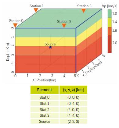
A correct analysis of the independent and joint effects of the parameters requires the evaluation of idealized scenarios where each variable can be properly controlled. Thus, the most relevant assumptions made in this initial analysis are: i) a horizontally layered earth model, ii) velocity increases with depth, iii) noise-free explosive point source filtered at 5Hz, and, iv) only one event occurs at a time. These assumptions are valid along this study unless otherwise stated. Although some of these assumptions are quite simple, they are a good starting point for further investigation with a more complex experimental setup.

The volume of study is a 5 km cubic layer cake model with velocities according to Figure 1. Moreover, the recording configuration consists of 4 equidistant stations in a square surface array

Figure 1 Layer cake velocity model and base case recording geometry. 

Even though BPI is suitable for location of a wide variety of seismic signals, as concluded in several studies [²⁴],[⁹],[³³],[¹⁷], the experiment proposed herein is designed to analyze local events only, at the small-scale of an oilfield or in the vicinity of a stimulated well. Furthermore, to make a clear analysis for each abovementioned parameter, wave propagation phenomena including scattering dispersion, attenuation, and anisotropic media are not considered in this study.

4. RESULTS ANALYSIS

Most seismic event location methods are vulnerable to instability and inaccuracy caused by changes in parameters such as velocity model, noise level, frequency content, and recording array configuration For some location methods, it is not straightforward to measure the impact of such parameters on their results. Fortunately, that is not the case for BPI, which allows to conduct robust sensitivity analyses as follows:

SIGNAL TO NOISE RATIO (SNR)

Methods using both the dynamic and kinematic wave information are quite stable in presence of high noise levels; however, decreasing the SNR may increase the number of artifacts and affect the resolution in the image domain. Hence, it becomes useful to pre-process data prior to further analysis in order to supress noise. Moreover, choosing a high threshold value (ɸ around 85%) also helps to discard highly energetic artifacts, without missing true sources with relatively low energy (Figure 2).

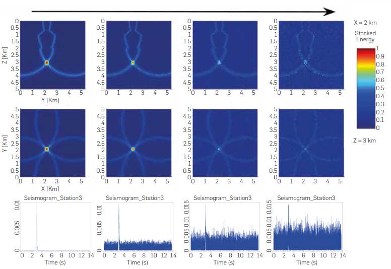
Figure 2 Influence of noise on spatial location of the event. Upper panel and middle panel show a vertical slice view (x-plane) and a horizontal slice view, respectively. The gradual increment of noise blurs the image; however, the true hypocenter is still well located. In the lower panel, their respective seismograms show a gradual increase of white noise from left to right. 

Backpropagating noisy seismograms may lead to increasing numbers of local maxima in the 3D space (x, y, z) as the level of noise rises. Nevertheless, the hypocenter is correctly located at (2, 2, 3) km when an appropriate threshold is used.

VELOCITY VARIATIONS

An accurate velocity model is an essential input in seismic and seismology as it determines if a reflector or an event can be correctly located in depth. Unfortunately, there is never a complete understanding of the geology and physics of the subsurface, which Leads to large uncertainty in the distribution of properties such as rock velocity, density, resistivity, permeability, and many other. This issue is partly overcome by the inversion of measure data and prior information; nonetheless, these estimates are never perfect, thus uncertainty will persist. Note: Velocities in this section are expressed as percentage of the true value (100%).

EFFECTS OF VELOCITY ON ORIGIN TIME.

For an unknown origin time t ₀ [s], a search for the global maximum must be carried out, not only in a spatial 3D volume, but also for different time windows. Now, let us assume the hypocenter is known. Then, the effect of incorrect velocities on the origin time can be tracked by plotting the energy at source as a function of time (Figure 3). As expected, the brightness curves rise steeply as the time window approaches the origin time and fall immediately afterwards to a level determined by background noise.

Figure 3 Energy (brightness function) at hypocenter vs origin time for 5 velocity models. Percentages below 100% indicate underestimated velocity models, whereas percentages above 100% indicate overestimated velocity models. The use of noise-free impulsive sources causes the spike-like shapes of the curves. 

It is worth noting that lower velocities result in earlier origin times than higher velocities, since waves travel slower and need more time to reach the recording array (i.e. think of a bus that must reach its destination at 12:00, its departure time t ₀ would have to be earlier if traffic was heavy, because of a lower mean velocity) Another important feature of these curves is that using incorrect velocity models produce a mismatch between signals such that the highest stacked energy can only be achieved with the true model in green (100%).

EFFECTS OF VELOCITY ON SPATIAL LOCATION.

For a known origin time t ₀ [s], reducing the values of the velocity model focuses energy at a shallower position than the true hypocenter. Conversely, overestimating the velocity model deepens the source (Figure 4). In addition, in the xy-plane at true depth (z=3km), the wavefronts travelling at lower velocities have not yet focused at the hypocenter, while at higher velocities, they have propagated beyond the hypocenter.

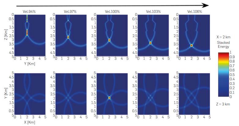
Figure 4 Velocity influence on spatial location of an event at the center of a square array (source 1). The upper panel presents a vertical slice view for 5 velocity models increasing towards the right. Notice that the use of incorrect velocities may produce artifacts (e.g. the Vel.94% model generates a near surface false candidate). The lower panel shows horizontal slice views at Z=3km. At this depth, only the correct model (Vel.100%) locates the source. Nevertheless, it is important to keep in mind that the other velocity models also focus coherent energy, but at different depths. 

Notice that the source only displaces vertically because of the symmetry of the recording array with respect to the source, indicating a trade-off between depth and velocity.

FREQUENCY CONTENT

As in the case of noise, peak frequency of the signal plays a key role on the resolution with which the source can be resolved. According 4.00 to Figure 5, the lower the frequency of the signal, the larger the zone within which the source can be located. This happens because Lower frequencies have longer wavelengths resulting in gradually Less capability to detect small underground features.

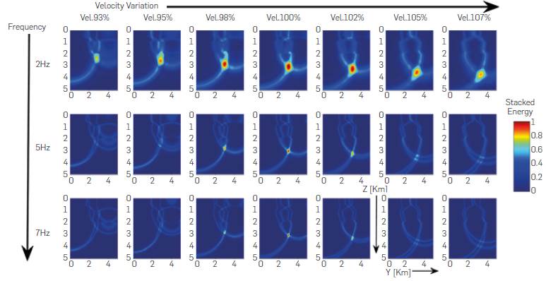
Figure 5 Non-centered event: Effects of frequency content and velocities on stacked energy. Vertical slices for 2Hz, 5Hz and 7Hz in the upper, middle, and lower panels, respectively. The Back-projection of low frequency signal is more stable and provides a first estimate of the solution, albeit care should be taken to prevent misclassification of false candidates as the true hypocenter. On the other hand, the use of higher frequencies helps to discriminate between true and false sources. 

This example summarizes the combined effects of frequency and velocity on stacked energy for a non-centered event beneath a square geometry. It should be kept in mind that trial velocities are presented as percentage of the correct velocity model (vel 100%). It is evident that back-projecting low frequencies can focus more energy for a wider range of velocities, thus being more stable for location. However, it may also produce false candidates (e.g. vel107% in Figure 5) that disappear as frequency content is higher, thus gaining in resolution. On the other hand, the downside of using higher frequencies is that a more accurate velocity model is required for the signal to add coherently.

GEOMETRY OF RECEIVERS

The accuracy of the spatiotemporal location (x,y,z,t₀) is partly dependent upon the array geometry and the relative position of the event source. Thus, a good surface coverage is mandatory for correct identification, location, and characterization of both active and passive seismic events.

An infinite number of possible configurations can be deployed on field during seismic surveys, and each one will imply different constraints on location accuracy. In this study, we are interested in assessing the impact of some basic array geometries, number of receivers, and relative position of the event on the location outcome of BPI.

Square geometry (Relative position of event)

Two experiments are carried out to evaluate the influence of the relative position of the event with respect to the recording array (Figure 6).

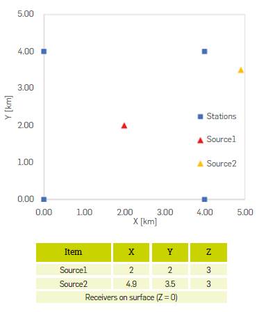
Figure 6 Square receiver geometry and relative position of 2 sources. Source 1 is located right underneath the center of the recording array. Source 2 is located outside the array. 

Source 1 - red triangle. This event is placed in the center of the array. The X and Y coordinates are perfectly retrieved with 0% error because of symmetry effects, regardless of the velocity and frequency used in the back-projection (as seen in Figure 7a). On the other hand, error in the Z-component varies significantly with velocity changes and reaches a value of up to 50% error for a -10% velocity variation. Additionally, the impact on t ₀ can be tracked with a curve called Maximum Brightness Function Curve (MBFC) which displays the maximum value of stacked energy in volume per timestep (Equation 5). This curve grows up as the back-projecting time-window approaches the true origin time thus giving a quick estimate of t ₀ .

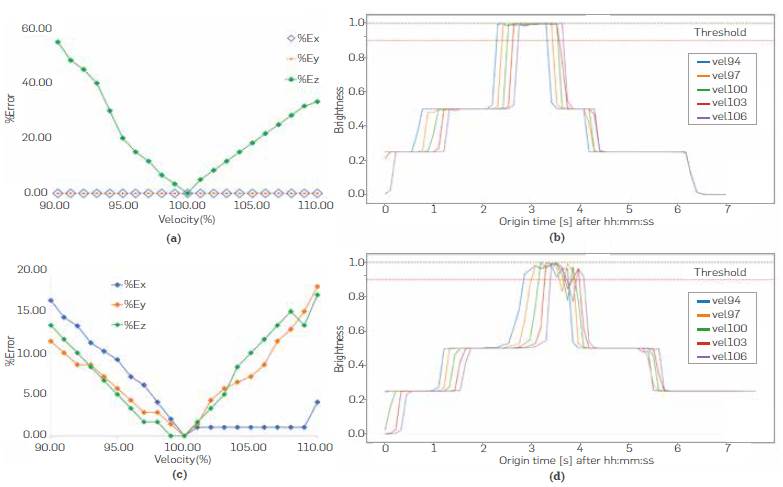
Figure 7 Solution accuracy vs Velocity. Source 1 in upper panel: (a) Percentage errors of the spatial coordinates for 21 velocity models, (b) MBFC vs time for 5 different velocity models. The red dashed line represents an arbitrary threshold to distinguish between false and true sources. These curves exhibit troublesome large plateaus that complicate origin time estimation. Source 2 in lower panel: (c) Percentage errors of the spatial coordinates of an event whose epicenter lies outside the recording array, (d) MBFC vs time for 5 different velocity models. 

It is evident in Figure 7b that lower velocities imply earlier origin times, as discussed earlier. Another interesting feature is the presence of a plateau that raises some uncertainty about the origin time. In general, the shape of the MBFC and its plateau length depend on numerous factors that include: i) dominant wavelength ii) frequency content, iii) spatial discretization of the grid, iv) timestep and time-window length, v) receiver geometry, v) noise level, and vi) source wavelet.

Source 2 - yellow triangle. For events originating outside the recording array, errors in X and Y become as large as depth errors (15% for a ±10% ΔV) (Figure 7c), and they continue growing as the hypocentral distance increases, together with a larger azimuthal gap. Likewise, the MBFCs in Figure 7d display slightly less symmetry, especially along the plateau where a notorious drop of energy occurs between 3.5(s) and 4.0(s). The staircase shape ndicates when one or more stations start or stop contributing to the energy summation.

During the back-projection, an overestimated velocity model may prevent energy from focusing inside the volume of study, even for events simulated inside the volume (upper panel Figure 8). Conversely, an underestimated velocity model may locate an external event inside the volume of interest thus leading to erroneous interpretations. This remark is of especial interest to microseismicity monitoring applications where high accuracy is required to discriminate induced from non-induced events.

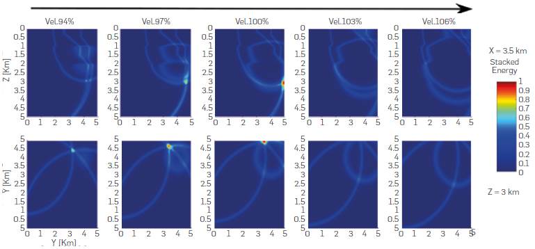
Figure 8 Source 2. Velocity influence on the spatial location of an event outside the recording array. The upper panel presents a vertical slice view at Y = 3.5km for 5 velocity models increasing toward the right. Unlike source 1, the event does not deepen vertically but diagonally until the energy no longer focuses inside the volume of study. The lower panel exhibits horizontal slices (Z = 3km) of the same volume. 

SQUARE ARRAY: NONLOCAL SEISMIC EVENT.

One extra scenario for the square configuration is presented in Figure 9 to complement the study on location accuracy of events originated far from the array.

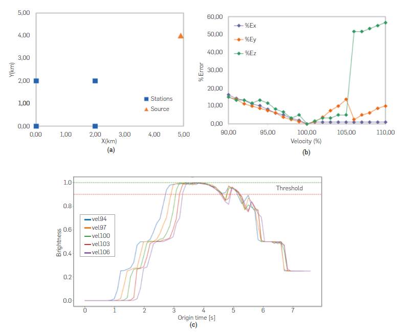
Figure 9 Solution accuracy vs Velocity for a nonlocal event, (a) source -receiver configuration, (b) Percentage errors of the spatial coordinates for 21 velocity models. For velocities in the range of 100%-105%, errors in the y-coordinate are larger than errors in X and Z. However, as velocities continue increasing, the true source energy leaves the volume of interest as it surpasses the model boundaries and, consequently, it is substituted with an incorrect maximum, (c) MBFC vs time for 5 different velocity models. These curves are similar in shape to those seen for source2; nonetheless, they exhibit larger plateaus that further complicate origin time estimation. 

This source is simulated at a distance from the array center of 2.5 times that of the side length of the square, which suffices for our purpose, considering our scale of investigation and interest in local events such as those detected in the vicinity of wellbores during microseismic monitoring.

The Back-projection shows that using underestimated velocity models produces location errors below 15% for the three spatial coordinates (Figure 9b), close to those obtained for source 2 in (Figure 7c). Likewise, an overestimation of the velocity model leads to a gradual increase in errors. For velocities above 105%, the true source leaves the volume of interest (see Figure 10), which may lead to an erroneous maximum found anywhere else within the volume.

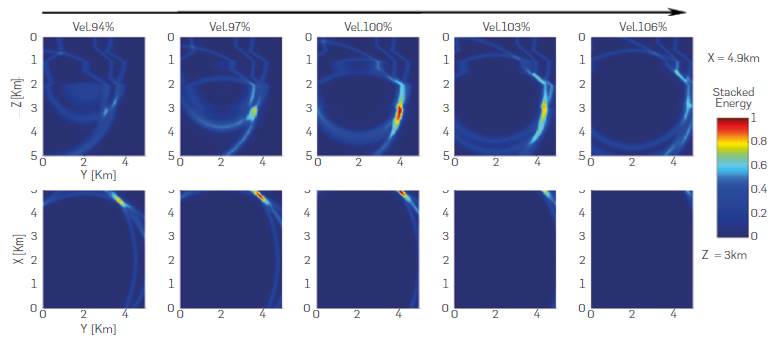
Figure 10 Velocity influence on the spatial location of a non-local event. The upper panel displays a vertical slice view at X = 4.9km for 5 velocity models. The source moves to the right as velocity goes up, until a point where the source energy is removed from the volume. The lower panel exhibits horizontal slices (Z = 3km) of the same volume. In this view, the energy moves diagonally to the top right corner before leaving the volume. 

It is clear from Figures 7d and 9c that the longer hypocentral distance of the last experiment adds more uncertainty in origin time estimation. A plateau on the MBFC that becomes longer as the source moves away from the array, indicates a trade-off between the hypocentral distance and the origin time, which in addition, is concurrently affected by velocity.

Circular geometry (12 stations).

This typical geometry consists of a circular array around the source which should facilitate its location. In seismology, a smaller azimuthal gap implies lower location uncertainty. For this experiment, a 12-station circular geometry is simulated with an azimuthal gap of 30° (as seen in Figure 11a).

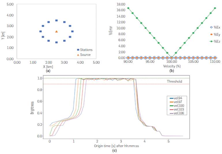
Figure 11 Solution accuracy vs Velocity using a circular recording geometry and a centered source, (a) Experimental setup, (b) Percentage errors of the spatial coordinates vs Velocity. Like sourcel in Figure 7a, a centered event enables x and y coordinates to be retrieved without error and, yields z-errors symmetric with respect to the vertical line vel=100%. (c) MBFC vs time for 5 different velocity models. Again, these curves are similar in shape to those seen for sourcel (Figure 7b), but with the largest plateaus among all the geometries studied herein. 

This configuration allows to recover the X and Y coordinates with total accuracy, which is a consequence of the symmetry of the source - array system. On the other hand, error in depth (Z-coordinate) behaves linearly with velocity, showing a maximum error of 17% (Figure lib). Additionally, the MBCs of the 5 velocities (Figure 11c) are not useful for origin time estimation as these curves have large plateaus with multiple local maxima.

Finally for a centered event in a circular array (Figure 12), the location is perfectly constrained laterally, and the source deepens vertically with velocity increments. Like the square array, this configuration is recommended for spatial location, although the origin time may require some extra analysis for more precise calculations.

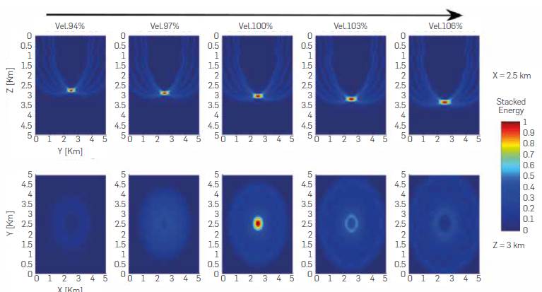
Figure 12 Velocity influence on the spatial location of an event in the center of a 12-receiver-circular array. Vertical slice views at X = 2.5km in the upper panel. Source deepens vertically, and there will be a significant trade-off between depth and origin time. Horizontal slices (Z = 3km) in the lower panel. For t_0, only the correct velocity model locates the source at the right depth, the other velocities locate it either at smaller or greater focal depths. 

LIMITATIONS

We point out that this manuscript sets a starting point for more complex scenarios to be tested. Further research may include, more realistic 3D velocity models and noise models, robust assessment of velocity uncertainty, recording geometries, different source wavelets, and spatiotemporal resolution in presence of more than one event.

We consider that, under the linear model for seismic wavefield, more complex signals like simultaneous microearthquakes and tremors can be understood as the superposition of impulsive signals. Therefore, we intend to cover hereunder the most fundamental principles of seismic event location under simple and controlled scenarios, where the effect of each parameter can be isolated and evaluated, so that these findings can be extrapolated to the application and interpretation of complex experimental setups in future research.

CONCLUSIONS

A lower peak frequency of the signal increases the stability of the BPI method and gives a reasonable first estimate of the solution, which can be further refined using higher frequencies with more accurate velocity models.

There is a trade-off between hypocentral distance and origin time. As the hypocentral distance increases, the MBFC exhibits a longer plateau, thus indicating a larger uncertainty in origin time.

There is a trade-off between origin time and velocity. For a known spatial location of the source, back-projecting with lower velocities result in earlier origin times than higher velocities as waves travel slower and need more time to reach the recording array.

There is a trade-off between hypocentral distance and velocity. For a known origin time, an underestimation of the velocity model produces a shallower hypocenter, while higher velocities deepen the event.

Although BPI is robust to low SNR, noisy data can significantly increase the number of artifacts and false candidates, thus, prior data conditioning is suggested to supress noise and enhance signal coherence among stations.

An incorrect velocity model prevents the stacked energy from focusing and reaching a reasonable maximum value, which might result in missed events.

It was observed that a good azimuthal coverage reduces the location error of seismic events. Additionally, depth appears to be the most sensitive spatial coordinate to velocity changes when the event originates inside the recording array.

BPI is a useful technique for location and detection of earthquakes and more complex seismic phenomena with no distinguishable seismic phases where picking of arrivals is difficult.