


 English (pdf)
 Article in xml format
 Article references
 Send this article by e-mail
 Cited by SciELO
  Cited by Google
  Similars in
SciELO
Similars in
SciELO  Similars in Google
 Permalink
1. INTRODUCTION
Offshore oil production and tanker transportation has increased since the 90s due to worldwide demand, and reduction of onshore reserves. These activities are associated to high risk as oil could be spilled accidentally into the ocean and, in certain situations, cause environmental, social, and economic impacts (Keramea etal. [1]). Oil spills are relatively common, and they occur in many ways, including natural releases. Most of them are small and occur, for instance, while refueling a ship or from oil leaks in transportation tankers. Although small, these spills can still cause damage, especially if they reach sensitive environments like beaches, mangroves, and wetlands. Large oil spills are dangerous disasters. These tend to occur during oil drilling, accidental collision, or sinking of oil tankers, and failure in pipelines and oil rigs. Consequences for the ecosystems and national and private economies can last for decades (Singh et al. [2]).
Singh et al. [2] prepared a map of potential oil spill risk for the Caribbean, pointing out that approximately 83% of the total area is exposed to some level of risk due to oil spills. Moreover, their quantitative analysis shows, in terms of crude oil tanker transport, that the islands, and Central/South American countries Exclusive Economic Zones (EEZs) are areas at moderate to high levels of risk. For oil products transport, the islands EEZs are generally at low risk levels, while South American countries are at low to high risk. The area between Colombia and Jamaica require close attention, as there is very high risk for pollution from the transport of crude oil.
In the Colombian coastal area over the Caribbean Sea, particularly in the Gulf of Morrosquillo, minor oil spill incidents have often been reported in the past. Based on reviewing national news and reports from environmental and maritime authorities, at least 9 oil spill incidents have been reported in this coastal area during the past 20 years (Table 1).
Table 1. Review of oil spill contingencies that occurred in the Gulf of Morrosquillo from 1992 to 2021
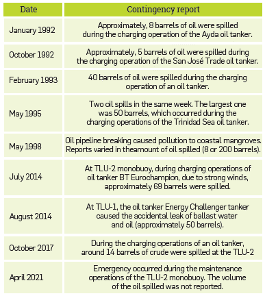
Most of the reports and information regarding the environmental and socioeconomic impacts of these incidents coincided that the established contingency operations designed to control the spills must be improved, to achieve better response after an oil spill initiated. This situation could be improved by means of numerical models which can be used for operational purposes.
To efficiently predict the trajectory and fate of hydrocarbon spills occurring at the sea surface, we simulated the movement, evolution and weathering processes of the floating chemicals released during two documented oil spills that occurred in the Maritime Oil Terminal of Coveñas. The oil spill model applied in this study can be used either in hindcast mode, capable of tracing the source of a spill, or in forecast mode, predicting the path, the horizontal dispersion, and the mass balance, assisting in this way to both contingency planners and pollution response teams during real-time crisis management.
2. OIL SPILLS BACKGROUND
The behaviour of an oil spill in the marine environment depends on a series of physical, chemical, and biological processes that are largely determined by the properties of the leaked oil, the hydrometeorological conditions (wave, winds, currents, solar radiation, sea water properties, etc.), and the characteristics of the release into the aquatic environment (instantaneous/continuous, surface/deep-water). From the moment the oil spreads over the seawater, oil properties (density, viscosity, etc.) change. This process, called oil weathering, refers to the changes that occur to oil as it stays in the environment. After the oil is released, it undergoes a wide variety of physical, chemical, and biological processes that begin to transform the oil almost immediately. [1].
In general, weathering processes can be analyzed in two different time-response windows. First, processes such as spreading, evaporation, dissolution, dispersion, and emulsification are rapidly occurring (within hours), and have immediate effects on the oil slick. Second, sedimentation, biodegradation and photo-oxidation occur more slowly (within months) and comprise the long-term mechanisms for the breakdown of hydrocarbons in the environment. Sedimentation, stranding, turbulent mixing, dispersion, and resurfacing are important processes, under distinct environmental conditions [1].
Spreading refers to the creation of a thin film that expands over the sea surface, as soon as oil is being released due to mechanical forces. Gravity and surface tension are the main forces acting in favour of spreading, while inertial and viscous forces are acting against it. Therefore, oil slick spreading occurs even in the absence of currents or deformations caused by wind. The spreading rate depends on the sea surface temperature (SST), oil viscosity, and density.
The horizontal transport of oil spilled at sea is largely determined by ocean currents, waves, and winds. Ocean currents and the wave-induced Stokes drift vary with depth, and the wind drag is commonly assumed to only affect the surface slick (Reed et al. [6]; Drivdal et al. [7]; Röhrs et al. [8]). Advanced oil spreading algorithms consider processes such as wind shear stresses, turbulent mixing, and wave breaking and shear spreading. Spreading is usually a process with specific model limitations, as it depends on oil characteristics and ocean conditions, and existing algorithms approximate only partially the actual surface area of real spills [1].
Horizontal transport includes both spreading and advection, which depend on currents, waves, and winds. Vertical transport involves vertical dispersion and wave entrainment, turbulent mixing, and resurfacing. The common modelling technique, employed by nearly all oil spill models is the Lagrangian approach, in which oil particles experience an advective displacement according to currents, wind and Stokes drift, and a diffusive displacement given by a random walk model.
Natural vertical dispersion is another significant process in the first week after an oil spill. This process deals with the amount of crude oil that migrates towards the water column in the form of small droplets because of turbulence, mostly produced by breaking waves. This process can have a significant effect on light crude oils under high turbulence. After evaporation, dispersion is the process with the most significant impact on the extent of time that the oil slick remains on the surface. Dispersion, however, does not produce changes in the physicochemical properties of the spill, as oil droplets migrating to the water column have the same chemical composition as the surface oil (Ramírez-Hernández, 2014 [9]).
Evaporation is an important weathering process, which removes the volatile elements of the oil to the atmosphere within a few hours of the spill, leading to the reduction of oil toxicity in the marine environment. In the first few days after an oil spill, the light, medium, and heavy crude oils can evaporate respectively up to 75%, 40% and 10% from their original mass (ASCE [10]). Simultaneously, the viscosity of the remaining slick increases leading to severe physical and chemical effects on the marine ecosystems. The most widely used analytical method to assess the rate of evaporation is based on the work of Stiver and Mackay [11]. The authors assessed oil evaporation by means of a mass-transfer coefficient, expressed as function of wind speed, oil spill coverage, oil vapor pressure, and sea surface temperature.
Emulsification is the process by which water is being mixed into the oil. This occurs when the water uptake increases. As the water fraction increased, the emulsion stability also increases. Note that the mass of the oil is the mass of pure oil. The mass of oil emulsion (oil containing entrained water droplets) can be calculated as: mass oil / (1 - water fraction). In general, water fraction = 0 means pure oil; water fraction = 0.5 means mixture of 50% oil and 50% water, and water fraction = 0.9 (which is maximum) means 10% oil and 90% water (Dagestad et al. [12]).
This water-in-oil emulsion in the form of suspended small droplets is often referred to as mousse. It occurs due to wave breaking, inducing sea surface turbulence, while oil composition, temperature, and viscosity play a significant role in the process (Mishra et al. [13]). The main effect of emulsification is that it creates an emulsion of considerably increased viscosity, compared to the oil initially spilled, resulting in serious implications for treatment methods. Another important negative effect of emulsification is that it increases the volume of the slick; this means that the clean-up costs are greatly increased.
Thus, emulsification is a process with specific model limitations and a crucial role on the impact assessment and response in oil spill modelling. A simple emulsification algorithm has been developed by Mackay et al. [14]. This model assumes that the rate of water uptake by the oil slick follows a first order kinetics with respect to the ratio of the current and the maximum water content. This rate law involves variables as wind speed, the fraction of water in the crude and the maximum water content that can support and stabilize the oil slick [9].
Photo-oxidation, biodegradation, and sedimentation are processes that occur in a later stage of a spill and are considered unimportant over the first days of a spill but become visible after a week or more. These are longer term processes that will determine the fate of the oil spilled [1]. Oxidation occurs when oil under the influence of the sunlight generates polar, water soluble, oxygenated compounds, generating tar balls that can accumulate in bottom sediments or along the coast. Even though this process is very slow, and it is not usually included in modern oil spill response models, under high UV light exposure, it can be fast, thus contributing to emulsification (Ward et al. [15]).
Biodegradation of oil by organisms is one of the natural processes that can attenuate the environmental effects of marine oil spills in the long term. The biodegradation rate depends on the type of hydrocarbon, temperature, species of marine micro-organisms, and availability of oxygen and nutrients. Biodegradation was generally considered a long-term oil weathering process, having a significant impact only after the first seven days of a spill and with time scales reaching up to several months; however, under specific conditions, it can become a significant process at shorter time scales, within the first week of an oil spill [15].
Sedimentation of oil droplets occurs because of three processes: increased density of the entrained oil and surface slicks due to weathering processes; incorporation into marine snow by means of zooplankton faecal pellets, or oil adherence or flocculation and agglomeration with suspended particulate matter (SPM) aggregates. This process causes several impacts on the marine environment, so it is material for biological impact analysis. Due to knowledge gaps in properly expressing the detailed dynamics of sedimentation in a quantitative parameterization scheme, this process has not been incorporated in oil spill models [1].
3. OIL SPILL MODELLING
Since 1960s, numerous oil spill models have been developed aimed at predicting the trajectory and fate of hydrocarbon spills occurring at the sea surface and the water column. These models, developed by various organizations, companies, and researchers, vary in complexity, applicability to location, and ease of use. The main inputs in each case are not only oil spill data, such as the type of oil and the initial location of spillage, but also metocean variables, such as the three-dimensional flow field, sea temperature, salinity and density profiles, atmospheric winds, and bathymetry, which may be obtained from different operational oceanographic forecasting systems available worldwide. A critical review of the state-of-the-art of oil spill models has been presented by Keramea et al. [1].
After a comparative assessment of the available models focused on supporting operational response to marine oil spill, we selected the oil drift module OpenOil, a 3D oil spill transport and fate model, which is based on the open source, Python-based, trajectory framework of OpenDrift ([8]; [12]). This system has been used by the Norwegian Meteorological Institute (MET Norway) for operational purposes as an oil spill contingency and search and rescue model, and for drifter and oil slick observations in the North Sea, being widely used by the scientific community in several oceanic regions (e.g., Jones et al [16]; Hole et al. [17]; Androulidakis et al. [18]; Brekke et al. [19]; Hole et al. [20]).
This model integrates algorithms with several physical processes, such as wave entrainment of oil (Li et al. [21]), vertical mixing by virtue of oceanic turbulence [21; Visser, [22]), resurfacing of oil due to buoyancy (Tkalich and Chan, [23]), and emulsification of oil properties [21]. Resurfacing is parameterized based on oil density and droplet size by means of Stokes Law, and, therefore, the model's physics are very sensitive to the specification of the oil droplet size distribution (Hole et al. [17, 24]). The oil properties in OpenOil are obtained from the ADIOS Oil Library [25], which is also open source, written in Python, and containing measured physical properties of almost 1000 oil types across the world [8].
The OpenOil model also supports oil spills back-tracking that simulates reverse scenarios to predict where an oil spill may have originated from, to investigate a spill of unknown origin, or for hydrocarbon exploration applications. As for oil transport and weathering processes, this model includes all basic processes such as advection, spreading, evaporation, dispersion, entrainment, diffusion, evaporation, biodegradation, and emulsification, following the Mackay's modelling approach for emulsification parameterization. A relatively sophisticated natural dispersion algorithm is included in OpenOil, principally computed via vertical mixing approach in combination with wave-breaking entrainment, and the option of different droplet size-distribution [8].
OpenOil includes parameterization of the oil weathering processes that are most relevant on timescale of hours to days, i.e., evaporation and emulsification. Dispersion is not treated separately in OpenOil because it is explicitly calculated by the vertical mixing scheme together with wave breaking entrainment, and droplet size distributions. The oil weathering calculation is based on the NOAA-ERR-ERD OilLibrary package, which is installed as a dependency. The code for evaporation and emulsification in OpenOil is taken from the NOAA PyGnome code and adapted to the OpenDrift architecture. The biodegradation process has been incorporated into National Oceanic and Atmospheric Administration (NOAA)'s GNOME oil spill model, by including a new biodegradation algorithm, which is dependent on the surface area of droplets (Thrift-Viveros et al. [26]).
Oil properties are obtained from the open source ADIOS oil database developed by NOAA [25]. This database is accompanied by a software library (written in Python, like OpenDrift) of chemistry and weathering algorithms, which are used to calculate the evaporation and emulsification of a given oil type.
The rate of evaporation varies strongly among various oil types and depends on the wind speed. Some oil types may be completely evaporated within a few hours, whereas others do not evaporate at all. More typically, 20%-40% of the oil (the lighter components) is evaporated within the first 6 to 12 hours. The rate of evaporation follows the Stiver and Mackay [11] approximation. This parameterization has been included in the ADIOS model (Lehr et al. [27]; Overstreet et al. [28]), developed by NOAA.
In addition to the removal of oil components from the sea surface, evaporation may also play an important role in the onset of emulsification, which has a very strong impact on oil viscosity. While some oils do not form water-in-oil emulsions, other oils only start to emulsify after some of the components have evaporated. The water content in the emulsion may then quickly rise from 0% at onset of emulsification, to a maximum level that is typically 80%-90% for most oil types in the ADIOS database [25]. The density of the emulsion thus gradually approaches that of water, but more importantly for transport and fate modelling, as well as clean-up operations, the viscosity may increase by several orders of magnitude [8].
STUDY CASE 1
One of the best documented events in the Colombian margin took place on 20 July 2014, when strong and sudden winds began to affect the charging operation of an oil tanker (BT Eurochampion 2004) at around 20:30 hours at the Tanker Loading Unit, (TLU)-2, located at 9.493° N, 75.776° W, at Coveñas (Figure 1). Due to the sudden extreme weather event, the company Oleoducto Central S.A. (OCENSA), in charge of the operations, authorized the movement of the tanker to the anchorage area to avoid a collapse against the monobuoy. Despite having suspended the loading operations, the intensity of the winds produced an abrupt and sudden tension in the mooring mechanisms of the tanker, causing the leakage of crude oil that was inside one of the transfer hoses. In this event, spilling of around 42 to 69 barrels of hydrocarbons was reported by the environmental agency of Colombia (ANLA [3]).
Once the climatic event ended, the next day (21 July 2014), OCENSA deployed personnel to secure and protect the monobuoy. The inspection concluded that there was no presence of crude oil around the terminal. The company and the Coveñas Port Authority made a helicopter overflight over the Gulf of Morrosquillo, observing an oil slick that moved in a north-northeast direction towards Palma Island. After confirming the location of the oil spill to the north from its origin, OCENSA immediately deployed the personnel, resources, vessels, and equipment required for in the contingency plan, which began with the installation of direct containment barrels at the point of detection of the slick. During the next two days, new overflights were made to locate the slick and conduct new spill containment measures.
On 22 July, new aerial inspections in the morning hours evidenced that the slick had changed its main direction, moving southeast, towards the Tolu municipality. The slick was observed near the El Francés sector, to the northeast of its original spill location. The same day in the afternoon, the community evidenced pollution to the north of El Francés sector, where numerous balls of solid crude, organic matter, and sediments where found.
The following days, these balls were also observed further north, up to the Berrugas sector, on the northern coast of the Gulf of Morrosquillo. On 23 July, tar balls were observed in the Zaragocilla sector. The next day (24 July), the cleaning operation of these tar balls continued in the beaches of Guacamaya and El Francés.
STUDY CASE 2
Another contingency occurred on 21 August 2014, when crude oil was being loaded to the Energy Challenger tanker in the TLU-1 monobuoy (9.496° N; 75.737° W), operated by Ecopetrol. The alarm was raised due to the presence of crude oil in the seawater.
On 22 August, a commission from the Regional Autonomous Corporations (CVS and CARSUCRE) along with Ecopetrol and OCENSA evaluated the situation and determined that a leak (fissure) in the ballast water system that is also filled with hydrocarbon was the cause of the spill of around 20 to 50 barrels of oil (CVS [5]). Through the overflight carried out later that day, the magnitude of the oil slick and its proximity to the beaches were evidenced. According to information from Ecopetrol officials, the slick was first observed approximately 3 km from the beaches of El Porvenir in the municipality of San Antero (near Coveñas). There were no further aircraft reports the following days.
Late on 23 August and the following day, there was plenty evidence of contamination on the beaches of Guerrero and Guacamaya (Tolú Municipality), both located a few kilometres to the north of El Francés sector. On 25 August, the local authorities declared public calamity, and on 27 August, these beaches were officially closed given that the oil slick detected was causing negative impacts on the tourism sector of the Gulf of Morrosquillo, as well as on small-scale fishing [4].
CONFIGURATION OF THE SIMULATIONS WITH OPENOIL
The OpenOil model version 1.5.3 was used to simulate oil spill trajectories in the Colombian Caribbean. Regarding the environmental input data, OpenDrift provides flexibility to use various configurations. In this study, oil particles are advected horizontally by ocean currents provided by the global ocean sea physical forecasting product PHY_001_024 of the Copernicus Marine Environment Monitoring Service (CMEMS), covering the Gulf of Morrosquillo at 0.083° (~9 km) horizontal resolution, with 50 geopotential vertical levels at hourly time steps. This analysis can be downloaded at http://marine.copernicus.eu/. The global and forecasting system uses version 3.1 of the NEMO ocean model. The physical configuration is based on the tripolar ORCA12 grid type. The 50-level vertical discretization retained for this system has a decreasing resolution from 1m at the surface to 450 m at the bottom, and 22 levels within the upper 100 m. Details of this product are described in Lellouche et al. [29].
Wind data were obtained from the global ERA-5 reanalysis provided by the European Center for Medium Range Weather Forecasts (ECMWF), which is hourly information at 0.25° (~27 km). ERA-5 is produced using 4D-Var data assimilation and model forecasts in CY41R2 of the ECMWF Integrated Forecast System (IFS). The reanalysis combines model data with observations from across the world into a globally complete and consistent dataset using the laws of physics. Data can be downloaded from https://cds. climate.copernicus.eu/. Details of this database are presented by Hersbach et al. [30].
Wave data is from the Marine Copernicus, global reanalysis WAV_001_032 (WAVERYS), which is 3-hour time step information at 0.2° (~22 km). The core of WAVERYS is based on the MFWAM model, a third-generation wave model that calculates the wave spectrum, (i.e., the distribution of sea state energy in frequency and direction) on a 1/5° irregular grid. Average wave quantities derived from this wave spectrum, such as the SWH (significant wave height) or the average wave period are delivered on a regular 1/5° grid with a 3-hour time step. WAVERYS considers oceanic currents from the GLORYS12 physical ocean reanalysis and assimilates significant wave height observed from historical altimetry missions and directional wave spectra from Sentinel 1 SAR from 2017 onwards. Variables used in the simulations are SWH and sea surface wave Stokes drift (u and v velocities). Detailed information of this dataset is presented by Law-Chune et al. [31]. The Stokes drift from surface gravity waves is treated separately in OpenOil and obtained from the wave model. Stokes drift below the surface is calculated from the surface Stokes drift using the parameterization provided by Breivik et al. [32].
It is important to highlight that it would be desirable to have meter-to kilometre spatial resolution forcing fields, but these are unavailable in this basin. Also, there were no available measurements of metocean variables during the time these contingencies occurred. Hence, the lack in situ or modelled data of higher resolution is a limitation identified in this study.
The simulations are initiated with 5000 oil elements (super particles) seeded at the ocean surface within the area of the TLU locations at the exact time and date when the reported incidents started. Since no reports regarding the type of crude involved in the spills is available, we chose Vasconia oil properties, similar to the medium crudes produced in the different fields of Colombia. Given the initial volume of oil spilled at the sea surface, for the first event (~69 barrels), a radius of the initial oil slick of 800 m was selected, while in the second simulation (20 to 50 barrels) the radius around the initial position is 400 m. given the initial volume of oil spilled at the sea surface. Note that the radius is not an absolute boundary within which elements will be seeded, but a standard deviation of a normal distribution in space. Thus, about 68% elements will be seeded within this radius, with more elements near the center. By default, elements are seeded at the surface (z=0). Outputs are set every 10 minutes until the simulation ends, which occurs when all the oil particles are deposited on the seabed, or over the coastline. The configuration features and the initial metocean conditions used in each experiment are summarised in Table 2.
Table 2 Configuration features of the two oil spill simulations performed in the Gulf of Morrosquillo with OpenOil.
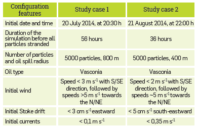
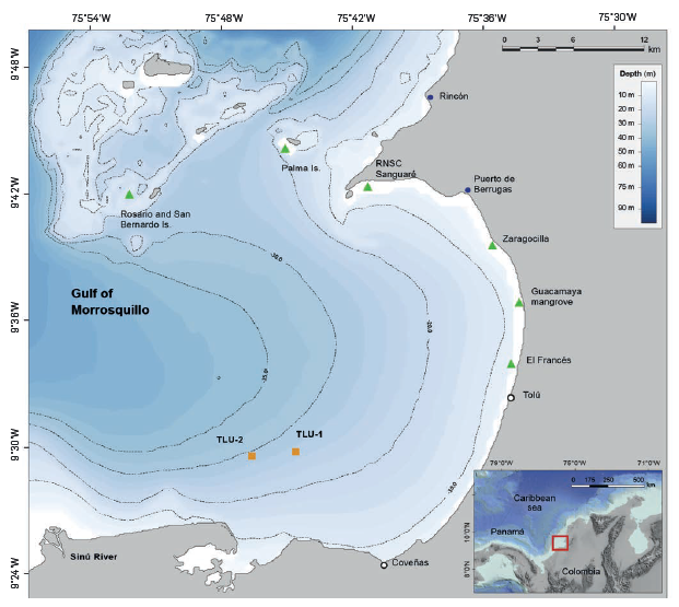
Figure 1 Gulf of Morrosquillo bathymetric map. The location of the Terminal Loading Units (TLU-1, TLU-2) of the Coveñas Oil Terminal is shown as full-orange squares. Location of the municipalities of Tolú and Coveñas (empty circles) and main beaches (full-green triangles) are also included. The regional context of the Gulf within the southwestern Colombian Caribbean is shown in the bottom right corner of the map.
METOCEAN CONDITIONS
The evaluation of the oil spill model outputs starts with the observation of the meteorologic and oceanographic (metocean) characteristics during the days the contingency occurred. These features that are used as inputs of the oil spill model are needed to understand prevailing conditions, and the main processes considered in the horizontal drift.
ERA-5 winds obtained from a location near the TLU-2 buoy show weak wind velocities (< 3 ms-1), and southward and south-eastward directions during the first hours of 20 July, followed by a northeastward direction and the intensification of the speed (>5 m s-1) during the afternoon hours (Figure 2A). The wind magnitudes from this reanalysis did not evidence the wind burst reported during the night, on 20 July, given that the reanalysis underestimates high wind speeds of short duration in this region (Devis-Morales et al. [33]). Winds at the time of the contingency (around 20:30 hrs) had a south-eastward direction, and the next day (21 July), the flow turned towards the north (northeast and northwest). During the following days, the winds tend to flow towards the south during the evening and morning hours, and towards the north during the afternoon hours.
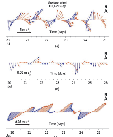
Figure 2 Time series of (A) magnitude and direction of the surface wind, (B) Stokes drift, and (C) surface currents from a location near the TLU-2 monobuoy during the first five days of July 2014 oil spill contingency. Blue (red) arrows represent the morning (afternoon) hours. Wind data are from ERA-5 reanalysis, wave data are from Wavery reanalysis and current data are from CMEMS.
Stokes drift (speed and direction) in the area when the contingency started followed the general wind patterns. Relatively small velocities (<3 cm s-1) were observed during the morning hours, and values increased during the evenings. At the time the event started on 20 July, the wave-driven flow had an eastward direction, and during the following hours switched towards the southeast and northeast (Figure 2B).
Surface currents on 20 July, flow towards the north-east during the hours prior and during the contingency (Figure 2C), with changes in the magnitude coinciding with changes in wind direction (Figure 2A). When the wind blows towards the southeast, ocean currents weaken, and when it flows towards the northeast, the currents strengthen in the same direction.
TRANSPORT AND FATE OF THE SLICK
The horizontal transport patterns of the oil slick clearly follow the wind and surface currents depicted in Figure 2A and 2C. The trajectory of the slick is advected towards the north during the first three hours of the simulation coincident with the direction of these forcing fields (Figure 3). Then, the particles started to move towards the east, and 24 hours later, the oil slick was advected to the northeast of its original position. Finally, the oil followed a south-eastward direction until it reached the central coast of the Gulf, in the Tolú Municipality, 56 hours later. The simulation ended on 23 July, 04:30 hours, when all the oil slick reached the coastline (stranded particles).
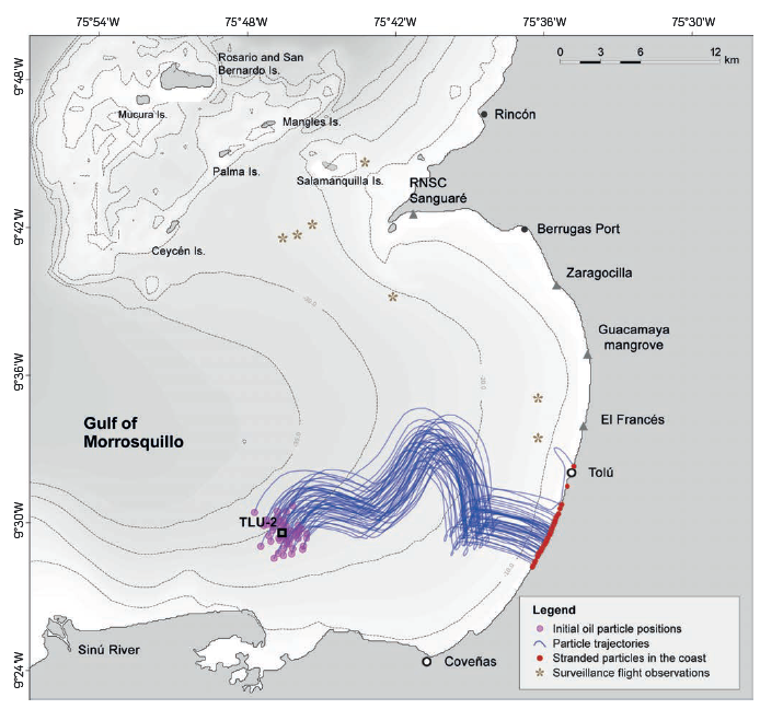
Figure 3 Oil drift simulation map starting at 20:30 h of 20 July 2014 and ending at 04:30 h of July 23, 2020. Location of TLU-2 (empty square), the initial oil particle positions representing the slick (magenta circles), the stranded particles in the coast (red circles) and particle trajectories (blue lines) are shown. Also, the position of the oil slick as reported from different surveillance flights in the area (stars) on 22 July are indicated (ANLA [3]).
The resulting trajectory differs from what was observed by the local authorities during the surveillance flights on 21 July. According to the reports, the oil slick moved further north, during the first 24 hours after the incident started, reaching the surrounding waters to the south of Palma Island (around 9.7°N) before advection occurring towards the southeast, towards the coast near the El Francés sector. The far north displacement of the slick was not well represented by the model given that the simulated slick advanced only up to 9.55°N. The differences encountered between air crafted observations and the simulation could be related to the horizontal resolution of the forcing fields (wind and waves) which is ~25 km. Also, as pointed by Devis-Morales et al. [33], the winds could be underestimated in this area, leading to the observed differences in the horizontal transport and fate of the oil slick.
OIL WEATHERING
The resulting simulation is analysed in detail by evaluating the spatial and temporal evolution of the oil evaporation and the water fraction. At the end of the first 24 hours after the simulation started, nearly 65% of the hydrocarbon was evaporated on the borders, and nearly 61% in the inner area (Figure 4A). As the oil slick continued moving towards the coast of Tolú municipality, the evaporation increased reaching 66% near the coast, at the end of the simulation.
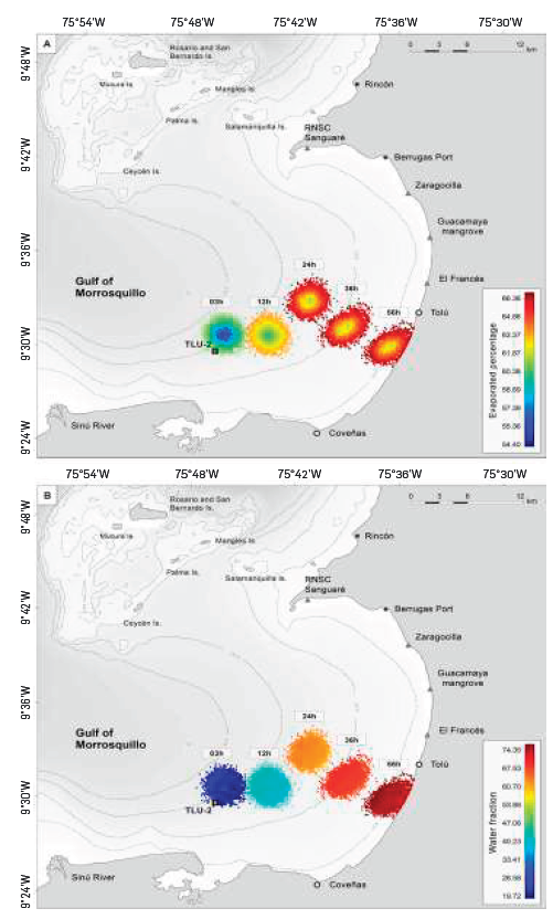
Figure 4 Evolution of (A) evaporated percentage and (B) water fraction within the oil slick. Simulation starting at 20:30 hrs of 20 July 2014, and ending at 04:30 hrs of 23 July, 2020, using 69 barrels of Vasconia oil spilled in the Gulf of Morrosquillo, in the location of the TLU-2 Coveñas Oil Terminal (square).
Evaporation rates resulting from this simulation are high and at first lead to interpret them as an overestimation. This has been previously discussed in detail by Ramírez Hernández [9], who developed an oil weathering model for Colombian crudes (MEUN). The author concludes that the evaporated fraction depends on wind velocities. For instance, with wind velocities above 5 m s-1 his weathering model for Vasconia oil tends to overestimate the evaporated fraction at the initial stages of evaporation (first 3 hours) but, with time (after the fifth hour), the difference between predictions and experimental data decreases. In the simulations performed in this study there were periods of high wind speeds; hence, it could be that the evaporation rates during the first hours of the simulations are overestimated. However, the emulsification of the crude oil is only possible when evaporation is large, thus, these rates are not excessively overestimated.
High evaporation values play an important role in the occurrence of emulsification, which has an impact on oil viscosity. In the case of the hydrocarbon spilled in this area, the slick reaches 74% of water content (fraction) when most of the oil (66%) has been evaporated. As discussed by Ramírez-Hernández [9] for Vasconia oil, these results represent the typical behaviour for oil emulsification, as it forms an emulsion with a water content of 70-90 % that becomes more stable as the evaporated fraction increases. As shown in Figure 4B, when simulation ends, the water fraction is nearly 75%, making emulsification possible.
These emulsions are referred to as "chocolate mousse" or "mousse", as they form a gelatinous emulsion of water and oil (Payne, 1982 [34]; Thingstad and Pengerud, 1983 [35]). This weathered emulsion then breaks into pieces, forming pelagic semisolid tar balls (Fingas and Fieldhouse, 2009 [36]). These balls were observed in the evening of 22 July, arriving on the coast beaches of El Francés, municipality of Tolú. The following days these balls were also observed further north, as far as Berrugas beaches, municipality of San Onofre, around 20 km north of Tolú.
Geographical location of tar balls, far north from where the open oil simulation ends, apparently contradict our results. We interpreted this difference as a limitation of the OpenOil model, which does not solve the coastal transport processes of the slick given that the simulation ends once oil particles reach the coast or settle on the seabed. Given that longshore coastal currents had a northward direction 24 hours after the simulation started, it is possible that tar balls that first reached the Tolú coast were advected along the coastline towards the north during the following days. The mass balance of the oil spilled on 20 July 2014, is shown in Figure 5. It evidences the rapid loss of the mass, during the first two hours after the contingency started (Figure 5A), because of the large evaporation (>50%) of the volatile fractions of the hydrocarbon. This process not only eliminates hydrocarbon from the sea surface to the atmosphere but is crucial in the changes the slick suffered in the next hours, given that the evaporation allows the gradual increase of the water fraction (Figure B), causing a large impact on the oil density (Figure 5C) and viscosity (Figure 5D).
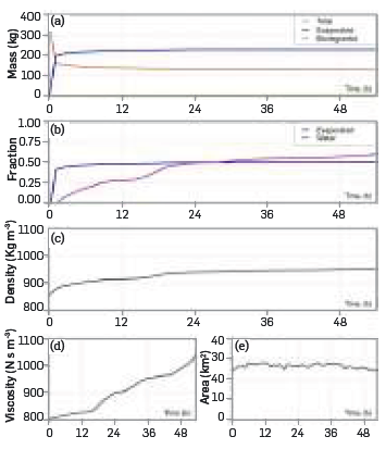
Figure 5 Mass balance of the Vasconia oil spill contingency that started on 20 July 2014, in the Gulf of Morrosquillo. It is shown the temporal evolution of (A) the total, evaporated and biodegraded mass (kg); (B) the evaporated and water fractions; (C) the density of the mass (kg m-3), (D) the viscosity (N s m-2), and (E) the area of the slick (km2).
The content of water in the emulsion changed rapidly from 0% at the start of the contingency to a maximum of 75% when it ended (Figure 4B and 5B). The density of the emulsion increased gradually to values near 950 kg m-3 (Figure 5C). Formation of TAR balls might also be supported by the fact that Vasconia crude forms a stable emulsion with a significant viscosity increase, once the evaporated fraction is over 15.5% [9]. That threshold is reached in one hour and that is why the viscosity increases just immediately after the spill started (Figure 5D).
Results obtained in this study matched the predictions of weathering for an oil spill of Vasconia crude oil with the MEUN model developed by Ramírez Hernández for the Caribbean Sea conditions [9]. Both simulations present a highly persistent behaviour of the crude on the surface, with a high evaporation fraction and less than 1% of dispersion because of the high viscosity produced by the stable water-in-oil emulsion it forms. The oil remaining on surface, after a spill of Vasconia, forms an emulsion with a water content that can be higher than 80%.
In this simulation the biodegraded mass is nearly zero for 56 hours (Figure 5A); hence, in this scenario there was no change of the total mass due to microbial degradation. Also, it was observed that the area of the oil slick remained relatively the same during the entire simulation. The horizontal spreading of the slick in this scenario was relatively small (Figure 5E) given that inertia and viscosity were the determinant mechanical forces working against the expansion of the oil film on the sea surface.
METOCEAN CONDITIONS
Metocean conditions during the contingency event are shown in Figure 6. At night, when the oil spill started (21 August, 22:00 hr), and next morning, winds had a south-eastward direction; then, there was a change in wind direction towards the northeast, which lasted the following days, with magnitudes around 5 m s-1 (Figure 6A). Stokes drift from surface waves observed during these days coincided with the wind direction, with maximum magnitudes of less than 5 cm s-1 (Figure 6B). Ocean surface currents in the area maintained a northeastward direction during the entire contingency event, with very weak magnitudes (close to zero) when winds turned towards the south, and maximum velocities (>0,35 m s-1) in days two and three of the simulation (Figure 6C).
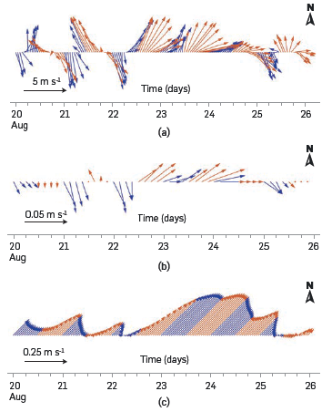
Figure 6 Time series of (A) magnitude and direction of the surface wind; (B) Stokes drift and (C) surface currents from a location near the TLU-1 monobuoy during the first six days on which the August 2014 oil spill contingency occurred. Blue (red) arrows represent the morning (afternoon) hours. Wind data are from ERA-5 reanalysis, wave data are from Wavery reanalysis, and current data are from CMEMS.
TRANSPORT AND FATE OF THE SLICK
The metocean conditions observed in the gulf favoured the oil slick to move northwards during the first three hours; then it was advected to the southeast, coincident with the change and strengthening of the wind direction (Figure 7). After 16-18 hours after the start of the simulation, the oil slick shifted its trajectory towards the north-east.
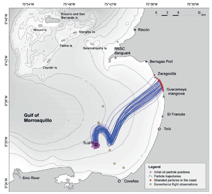
Figure 7 Oil drift simulation map starting at 22:00 h of 21 August 2014 and ending at 17:00 h of 23 August 2014. Location of TLU-1 (empty square), the initial oil particle positions, stranded particles in the coast (red circles), and particle trajectories (blue lines). Also, the position of the oil slick as reported from a surveillance flight of the area (stars) on 22 August is indicated.
Finally, the oil particles moved rapidly towards the central coast of the Gulf of Morrosquillo, until the slick reached the northern sector of El Francés, and the beaches of Guacamaya and Zaragocilla at, ~36 hours after the contingency started (Figure 7). Part of the simulated trajectories are consistent with the reports from the local authorities that monitored the oil slick from aircrafts on 22 August, and the information from the tourist sector that observed oil pollution on the beaches on 23 August. Discrepancies with some surveillance flight observations could be related to the resolution of the forcing fields or the underestimation of the wind velocities from ERA-5. Nevertheless, from these results, it becomes evident that the combined effect of the wind, the Stokes drift and surface currents in the same direction in day two were determinant in the rapid movement of the oil slick towards the northern coast of the Gulf.
OIL WEATHERING
The evolution of the evaporation and the water fraction within the oil is shown in Figure 8. It is observed that in the first three hours, 62% of the total mass was evaporated; after 24 hours, 78% of the crude oil was eliminated to the atmosphere, and 36 hours after the simulation started, 85% of the spill was evaporated (Fig 8A), inducing changes in the density and dynamic viscosity of the remaining mass, which, in turn, favoured the increase of the water fraction, from 4% during the first hours to 72% at the end of the simulation (Fig 8B).
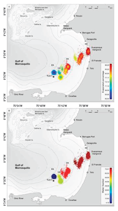
Figure 8 Evolution of (A) evaporated percentage and (B) water fraction within the oil slick. Simulation starting at 22:00 h of 21 August 2014, and ending at 17:00 h of 23 August 2014, using 50 barrels of Vasconia oil spilled in the Gulf of Morrosquillo, in the location of the TLU-1 Coveñas Oil Terminal (square).
During this contingency event, winds and currents were more intense than during the incident in July; hence, the evaporation rates were greater this month, allowing a rapid mixing between oil and ocean and the surfactant/stabilizing effect of certain compounds in the crude oil (mainly resins, asphaltenes and waxes), which facilitated the formation of water-oil-emulsions with up to 72% of water content.
The mass balance of the oil spilled in August 2014, is shown in Figure 9. In this event, the rapid decrease of the total mass due to evaporation is evident, which reached 75% in the first six hours (Figure 9A). As the evaporated fraction increased, this favoured the gradual increase of the water content (Figure 9B), and the density of the resulting mass, which increased to values close to 1000 kg m-3 (Figure 9C). Although the density increases, the slick remains superficial, increasing its viscosity (Figure 9D). With increasing evaporation and water content, the emulsion contributes significantly to the persistence of the slick, mainly due to the large increase in viscosity and thickness.
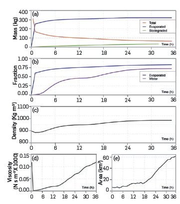
Figure 9 Mass balance of the Vasconia oil spill contingency that started on 21 August 2014, in the Gulf of Morrosquillo. It shows the temporal evolution of (A) the total, evaporated and biodegraded mass (kg); (B) the evaporated and water fractions; (C) the density of the mass (kg m-3), (D) the viscosity (N s m-2), and (E) the area of the slick (km2).
These weathering processes, together with persistent winds and currents favour horizontal spreading and, further, the increase of the oil spill area, which reached 60 km2 at the end of the simulation (Figure 9E). Once the spilled started its advection on the sea surface, strong metocean conditions caused the increase of the horizontal spreading of the slick. The temporal evolution of the oil slick has been discussed by Fay (1971) [37], who concluded that after the first hours of a contingency event, the extension of the slick becomes more affected by the influence of wind, waves, and currents.
In this event it was also observed that biodegradation processes started to occur, being evident 12 hours after the oil was spilled (Figure 9A). Nevertheless, values were relatively small. The degradation rates depend on the oxygen and nutrients availability and the water temperature, along with the characteristics of the crude oil and the size of the droplets. The weathering processes cause the increase in the area available for biological activity, which favours the biodegradation process. The simulation ended after 35 hours, when all the particles were evaporated, biodegraded, or finally reached the coast and became inactive in the simulation.
CONCLUSIONS
Given the environmental and socioeconomical hazards associated to hydrocarbon transportation, it is important to understand the behaviour of crude oil after the contingency event of an oil spill. The results of the application of the oil spill transport and weathering model, OpenOil, in the Gulf of Morrosquillo, Colombian Caribbean, were presented, considering two events occurred in July and August 2014. Although no satellite images of these contingencies were found, these events were adequately characterized by means of available secondary information (reports, news, etc.) so that the simulations conducted could be validated.
The evaluation of the oil spill simulations showed that the tools implemented in this study are adequate to simulate contingencies related to the hydrocarbon charging/discharging that takes place in the Coveñas maritime terminal. These provide valuable information on the path followed by the spilled oil and the temporary evolution of the weathering processes, according to local metocean conditions, and the type of hydrocarbon used.
Major differences between the position of the oil slicks observed in the Gulf and those simulated by the numerical model are explained by the resolution of the forcing fields. In this semi-enclosed basin, a higher resolution database is recommended. Given that available information needed to force this model has a horizontal resolution >9 km, it is necessary to implement 3D ocean models in this before simulating oil spill trajectories and weathering processes.
In the modelling approach, longshore currents, along with oceanic currents need to be considered in future experiments. This could improve the resulting simulations regarding the fate of the oil spill when it reaches the coastline.
It is evidenced that the wind and the current effects are main factors inducing changes in the position of the oil spilled in the Caribbean Colombian basin. Differences encountered in the forcing fields in both simulations could explain the horizontal spreading observed, resulting in variations in the oil slick areas. In the August simulation, both, winds and currents were stronger than in the July simulation, inducing an increase of the slick area.
Wind not only causes the horizontal advection and spreading the oil slick on the sea surface, but also influences physicochemical properties. There is evidence of a dependence of evaporation with wind velocity, and maximum water content depends on the evaporation. In the August simulation, winds were relatively strong; this could be the reason for the evaporated and water fractions being higher this month as compared to the simulation in July.
The wind data used in the oil spill and weathering model is important and should be cautiously selected. Underestimation of the wind magnitudes by the reanalysis products could have an important effect on the resulting simulations. Given that most reanalysis products have limitations in shallow areas, it is advisable to implement an atmospheric model in this region capable of solving physical processes at local scales. However, before more sophisticated models are implemented, it is very important to have a current, wave, tidal, and meteorological observation system that provides real-time data needed to validate reanalysis models or used as input information to run an operational model.
This first attempt to predict the fate and evolution of oil spilled in the Gulf of Morrosquillo allow us to conclude that this is a useful tool that could be used for operational purposes, if used with higher resolution forcing fields. Knowledge of the path of the spill, obtained from the OpenOil model implemented in this study, will enable the prediction of possible affected areas, and will help to design proper mitigation strategies and protocols, aimed at reducing the risks and negative impacts associated with this type of contingency.
There are no other oil spill simulations in this region for comparing, nor field data for the model results to be directly compared with observations; however, the results obtained by the OpenOil model are consistent with the physics of the problem and the chemical evolution of this type of oil spilled in the seawater. Nevertheless, the fate of the spills matched the reports from the local authorities that observed the oil slick from aircrafts or from the coast.
Limitations encountered in the global reanalysis models are the main source of discrepancies between the simulations and the observations of the oil slick position and transport processes. Currently, ongoing work at the ICP-Ecopetrol is focused on improving the local 3D air-sea interaction models to solve dynamic processes in the Colombian coastal region.

