


 Inglês (pdf)
 Artigo em XML
 Referências do artigo
 Enviar este artigo por email
 Citado por SciELO
  Citado por Google
  Similares em
SciELO
Similares em
SciELO  Similares em Google
 Permalink
1. INTRODUCTION
The Full Waveform Inversion (FWI) is a method aimed at setting geophysical models that can reproduce the observed data [1], [2]. The inverse problem consists in obtaining the parameters of the earth's model by using an optimization algorithm, generally, a method based on gradients [3]. The four main elements of the FWI are: the observed data, drived from a seismic survey over the area of interest and acquired by surface sensors; the mathematical operator used for wave modelling; the cost function, which measures the difference between the modeled and the observed data; and the inversion strategy that defines the adjoint and gradient equations to update the physical parameters.
One of the major challenges in FWI is the computational cost as each iterative update of the models requires computing the forward and adjoint wavefields. Hence, different techniques have been developed to solve this problem [1],[4],[5],[6]. This paper proposes a methodology that includes the detailed steps for the pre-conditioning of seismic data for FWI, which considers the features of acquisition geometry, source estimation, and first arrival tomography to estimate the initial velocity [7],[8] and density models. The steps for pre-conditioning the observed data are also included. The methodology also considers strategies for the software implementation, so as to meet the requirements of the FWI (memory and computer requirements for wave propagation, wave back-propagation, gradients, cost function and quality controls). Those strategies include the optimal advance (L-BFGS) at some iterations and the notion of replicas of the seismic processing, such that a computer equipment with low-to-intermediate specifications can run the 2D acoustic FWI process.
Data pre-conditioning is a crucial step during the FWI. It enables the selection and enhancement of the seismic events used to update the physical parameters during the inversion. Both, land and marine datasets, offer different interactions between surface and body waves. Therefore, the pre-conditioning process for each dataset must be different. In [9] , the authors present a methodology for FWI on marine datasets. In this paper, the step-by-step guide uses only refracted waves of a land dataset during the FWI, to avoid the ground roll noise present in reflections.
2. INPUT DATA SET
The SEAM Phase II Foothills project is a synthetic model created to include geological features in mountainous regions [10]. Some of the features are rugged topographies, surface and in-depth alluvial deposits, complex geological structures resulting from the compressive fold, and tectonic push during mountains building.
In this paper, the FWI uses a Dip 2D line of the SEAM Phase II Foothills project [10] to test its performance. The Dip line undergoes abrupt geological changes and rough topography. Thus, the FWI tests on the central 2D Dip line provide us understand the difficulties in the estimation of complex geological models. The central Dip line has a total of 194 sources and 387 receivers distributed over 14,5 km. The main feature of this arrangement is to emulate a low-resolution acquisition by its thick spacing between sources (75 m) and receivers (37,5 m), with a maximum offset of 3 km in a split-spread arrangement.
3. EXPERIMENTAL STEP-BY-STEP WORKFLOW
The proposed methodology for processing a 2D land seismic line is summarized in the following steps:
1. Load of the observed data and quality control (QC) of its geometry. The first step is to perform a quality control of the information in the headers of the recorded data, by contrasting it with the technical information described in the characteristics of the acquisition. Quality controls are focused on verifying that the positions of sources and receivers match with that described in the acquisition document. Regarding the experimental dataset, the reference information is given by the SEAM Phase II Foothills project [10].
2. First arrival picking for the estimation of the initial velocity and density models. The first arrival seismic tomography is used to build the initial velocity model. The Geotomo Tomoplus tool was used to find the initial velocity and density models of the Dip 2D line [16] . The principle of Tikhonov regularization was used to pick the first arrival and build the tomographic model [17]. For the 2D Dip line, the test requires 30 iterations, and the solution ranges between 600 m/s and 6.500 m/s (see Figure 2-Left) [18]. The density model for the Dip 2D line was obtained using the Gardner's rule [11] on the tomographic result of the velocity model, with values of α= 0,31 and β=0,25; and then scaled by 1.000 to leave the densities in Kg/m 3 (see Figure 2-Right).
3. Analysis of the frequency content of the observed data. This step includes the analysis and selection of the frequency ranges to be used in FWI for all shots. It is necessary to choose a wave equation that incorporates the physical variables of interest and its subsequent discretization. In this case, the first-order acoustic 2D operator was chosen (Equation (1)) as the tool for simulating the propagation of the wave and generating the modelled data.
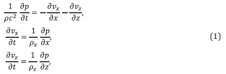
where p is the pressure field, c is the medium velocity and ρ is the density. The velocity of the particles in the x and z direction are v x , and v z , respectively. t is the time, and the density ρx is obtained by averaging ρ in the x direction while ρz is obtained by averaging ρ in the z direction.
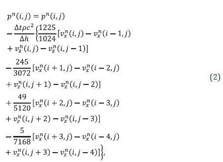
The discretized version of Equation (1) is given in Equation (2). The coefficients for an eighth order precision of the first derivatives are chosen for the staggered grid-centered approach [12].
where Δh=[Δx,Δy,Δz] is the spatial step and Δt is the temporal step.
The stability condition is achieved when the coefficients comply with the following equation [13]
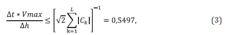
where Vmax is the maximum velocity of the propagation, L is the order of precision, and k is the number of coefficients or next neighbors in the nodes of the interleaved mesh, also called weighted C k .
In addition, the numerical dispersion is reduced by taking 4-8 points per wavelength. In this methodology, 5 points per wavelength are selected so that,
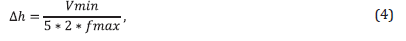
where Vmin is the minimum propagation velocity, and fmax is the maximum frequency of the source.
For the selected dataset, the minimum velocity in the model is that of the air layer with a value of 340 m/s. However, this value should be replaced by a higher value to avoid very fine spatial resolutions. Equations (3) and (4) were used to ensure stability and low numerical dispersion; with vmin = 836,4 m/s and vmax = 5.427,3 m/s. The discretization parameters can be seen in Table 1.
4. Source estimation. The Klauder's equation is used for the estimation of the source [10] (see Equation (5)), which center frequency and delay characteristics are estimated from the data. FWI requires starting with low frequencies, and increasing the frequency as the algorithm progresses [1].
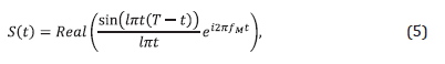
where the parameter l is the sweep rate (the change of frequency per unit time), while f M is the central frequency and T is the sweep length. The original source was filtered with an Ormsby bandpass filter [19] with cutoff frequencies [0-2-4-6] Hz, to limit its frequency content to a maximum of 6Hz with a 1ms sampling rate.
5. Filtering of the observed data. The filtering of the data keeps only the low frequencies on each shot. In this case, the observed data is filtered with the same filter used for the source. For the dataset, The same Ormsby bandpass filter of the source is applied to the observed data, with cutoff frequencies [0-24-6] Hz. This is to limit their frequency content to a maximum of 6Hz and eliminate all data elements observed that will not appear in the modeled data.
6. Generation of modeled data. Given the acoustic wave equation (see Equation (1)), the modeled data is obtained using the estimated velocity and density models and the estimated source. The depth of the velocity and density models were doubled and 30 air layer points were added to use the CPMLs [20]. The velocity in the air layer was modified to 900 m/s. This adjustment was also performed on the density models using Gardner's rule. Using the selected models, the modeled data is computed with an external module that performs the wave propagation.
7. Filtering of the modeled data. Once the modeled data has been generated with the velocity and density models, all shots are filtered so that the same bandwidth as the observed data is obtained. For the dataset, an Ormsby bandpass filter with cutoff frequencies [0-2-4-6] Hz is applied to the generated data and resampled at 8ms, for comparison with the observed data.
8. First arrival time adjustment. The adjustment of the first arrivals t 0 in the observed data is required to match the arrival time of the modeled data and to avoid cycle skipping. This adjustment should be done because during the modeling stage the source is ideal and the first arrival of the wave along with the response of the receivers is immediate. In the observed data, however, this behavior is affected by the response of the instruments and by the synchronization of the loads in the field. In the dataset, the time shifts are obtained manually by visually comparing the shots. The time shift was applied to the observed shots using the modeled data as a reference. To implement these shifts, the replica notion was used.
9. Creating/applying top and bottom mutes. Top and bottom mutes are required to remove those events that will not be considered for FWI. For this work, the spatial mutes from the seismic processing tool are used, performing a manual picking. The top mute is used to eliminate noisy events present in the observed data, which are located above the first arrivals. On the other hand, the bottom mute is used to eliminate all events that differ from refracted waves (ground roll noise, reflected waves, etc.). In this case, the top and bottom mute were created from the observed data, and the same was applied to the modelled data.
10. Selection of offsets. The cross-correlation on modelled and observed data allows identifying the offset intervals with cycle skipping that cannot be used during the inversion and to review similarities between events as the offset changes. The cross-correlation is intended to measure the time lag between the two data sets to thus identify the possible cycle-skipping and their evolution per iteration.
Once the offset ranges are identified, they are extracted per shots and saved as .csv files. First, the modelled shots are subtracted from the observed ones. Then, the channels in the CPML zone are marked so that they are not considered during the FWI. Lastly, it turns off the information per shot outside the offset intervals chosen in the .csv file. This ensures that only those parts of the residuals that meet all the recommendations are used.
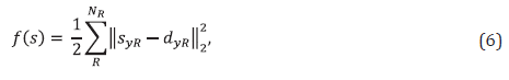
11. Evaluation of the cost function. For the first iteration, the cost function is assessed using the initial velocity and density models. This step is part of the elements for the quality control of the waveform inversion as it allows inspection of the evolution of the cost function. The cost function indicates the number of iterations needed by the algorithm. At each iteration step, the following equation is used where, s yR is the modeled pressure field measured at the receiver's location and d yR is the observed pressure field measured at the receivers location.
12. Adjoint fields. The computation of the adjoint fields is obtained using the adjoint equation (see Equation (7)) [14]and the residual fields obtained by subtracting the modeled data from the observed data
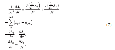
Where λ 1, λ 2 and λ 3 are the adjoint fields.
13. Gradient computation. The gradients of the physical parameters to be estimated [13] are defined as
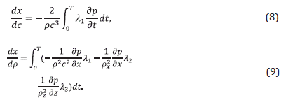
Once the forward and adjoint fields have been obtained, the next step is to find the product between those fields. As the calculation of the gradients involves the creation and storage of the adjoint and forward fields, the storage and RAM memory requirements of computer equipment can be unmanageable. That is why the replica notion was used to compute each gradient separately and in sequence. Finally, the gradients are added to build the total gradient, taking advantage of the superposition principle.
14. Velocity and density updates. This step is to update current velocity and density models using only gradient information (first iteration) or optimum advance [15] (starting from the second iteration). A topography layer is used to mute the air layer. It is also necessary to eliminate those pixels with a lot of energy to mask the information delivered by their neighbors. Those pixels are called outliers. These outliers are usually produced by the footprints of sources and receivers that produce high energy during the gradient calculation. To overcome this issue, it is recommended to create a mask for the outliers. Once the mask is applied on each gradient, the information provided by each vector shows the zone in depth that will be updated during the current iteration.
With the adjusted velocity and density gradients, the first update of the physical parameters is obtained. When only the first gradient information is available, it is recommended to use the steepest descent method [21]. With the new velocity and density values, the new gradients can be calculated. This allows using an optimal advance algorithm (L-BFGS). We proceed to the calculation of the attempts for an optimal advance where a value between 0 and 1 is required such that the cost function decreases. With the new velocity and density models, a new gradient is calculated, and the process is repeated until some stopping criteria are reached.
15. Quality control. This step performs a quality control on the new modelled data to verify the correct evolution of the velocity and density models.
The evolution of the offset intervals per shot using the cross-correlation can be used as quality control (QC) during the inversion process. This metric, unlike the cost function (which gives a general measure of the inversion process), allows to identify the evolution of each shot used in the full-waveform inversion process. The per-shot offset intervals are used to identify the residuals that will be used during the calculation of the adjoint fields. In general, it is expected that these offset intervals will expand as the iterations increases.
16. The steps 6 through 15 repeats to find new gradients. The stopping criterion is obtained when the comparison of offsets does not show an improvement and the cost function decreases very little; it is therefore recommended to extend the interval of offsets to incorporate new events per shot during the inversion process.
17. Steps 6 to 16 are repeated for the new group of offsets to find the new gradients. The stopping criterion is obtained when the comparison of offsets does not show an improvement and the cost function decreases very little. Then, it is recommended to extend the offsest interval to incorporate new events per shot during the inversion process.
18. Steps 3 to 17 are repeated to find the models for the next frequency range. The parameters to be used must be recalculated to guarantee the stability and numerical dispersion. The stopping criterion is obtained when there is no improvement of the comparison of offsets and the cost function decreases very little.
4. RESULTS
The Dip 2D line data has 194 sources distributed every 75m, and with a distribution of receivers every 37,5m. The elevations of the sources, receivers and CDPs (see Figure 1) are also verified. Figure 2-Left depicts the initial velocity model, and Figure 2-Right depicts the initial density model obtained by using Gardner's rule, with α = 0,31 and β = 0,25; and scaled by 1.000. Using Equations (3) and (4) with vmin = 836,4 m/s and vmax = 5.427,3 m/s, the discretization parameters are Δt = 1 ms, Δh = 12,5 m. Thus, first iterations will be able to resolve information with low frequency content up to 6,69Hz (see Table 1).
Table 1 Parameters used for the time-domain finite differences to guarantee stability and low numerical dispersion.
| Name | Vmin (m/s) | Vmax (m/s) | Δ t (ms) | Δ h (m) | Fmax (Hz) |
|---|---|---|---|---|---|
| Dip-vel-oo-3000 | 836,4 | 5.427,3 | 1 | 12,5 | 6,6912 |

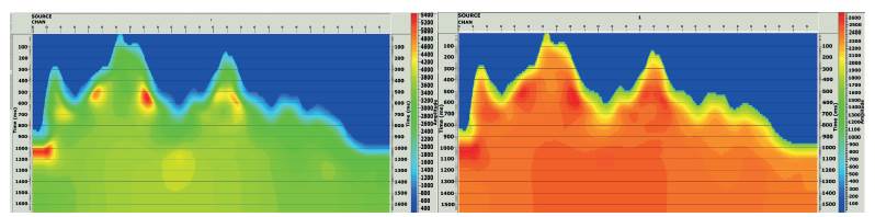
Figure 2 Left: Initial velocity model. Right: Initial density model obtained by using Gardner's rule, with α = 0,31 and β = 0,25 and then scaled by 1000
The original version of the source (see Figure (3)) is compared with the new source, showing a more limited frequency spectrum (see Figure (3)-right). Figure 4 illustrates the frequency content of shot 106 of the original 2D Dip line (see Figure 4-left) and the filtered shot (see Figure 4-right). Clearly, the frequency content of the shot is reduced (graph in red). For most of the shots, the original frequency content ranges between 5 and 35Hz. However, the main difference lies in the lower frequency. In some shots, the spectral content starts from 3Hz, while in others ,from 6 to 9Hz. Figures 5-left and 5-right depict the velocity and density models, where the depth was doubled, including 30 air points, with a wave velocity of 900 m/s.
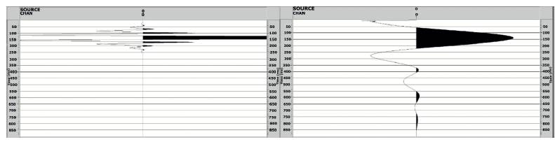
Figure 3 Source transformation. Left: Original source having 22.222 samples at 0,45 ms. Right: down sampled source having 10.000 samples at 1 ms.
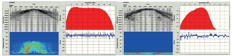
Figure 4 Shot 106 of the 2D Dip Line. Left: Original frequency spectrum. Right: Frequency spectrum filtered with an Ormsby filter [0-2-4-6] Hz.
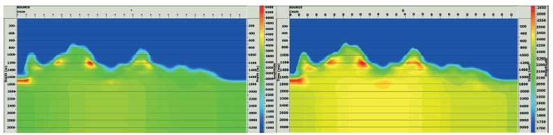
Figure 5 Left: Initial velocity model. Right: Initial density model. These models include 30 air points with a velocity of 900 m/s
Note in the filtered modeled data (Figure 6-Left) and the filtered observed data (Figure 6-right), that there are some similarities in the refracted events for certain offsets intervals. Therefore, it is necessary to identify the events that will be used for the calculation of the residuals.
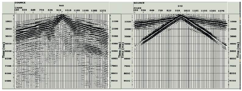
Figure 7 illustrates the time delay applied to the observed data shot 77. A time shift of 104ms was applied to the observed shots using the modeled shots as a reference. After adjusting first arrivals, those events that will not be considered during the full waveform inversion process are removed. Figure 8 illustrates the data observed after the effect of Top and bottom mutes. This same mute is applied to the modeled data.
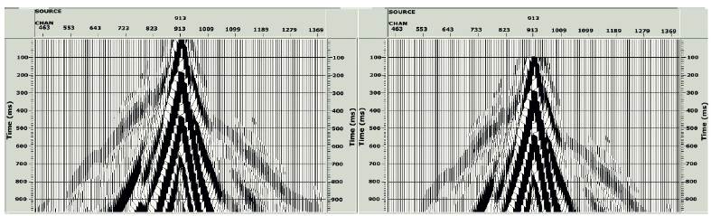
Figure 7 Shot 77 of the Dip line. Without time delay (left) and including time delay of 104 ms (right).
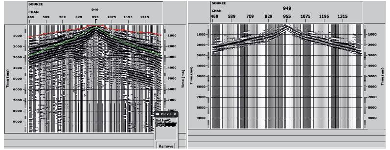
Figure 9 shows the cross-correlation between the modeled and the observed data. The horizontal axis represents the shots, the vertical axis represents the offsets, and the colors represent the time lag between both datasets. An interval of +55ms and -55ms was used. The intense green shade marks the areas with a 0ms lag and the intense red and blue shades mark the +40ms and -40ms gaps. Figure 10 shows the example of residuals for the shot 80. For the first offset interval, the residuals were calculated, and the first value of the cost function was found. Figure 11 illustrates the interaction of forward fields with adjoint fields for a single snapshot, highlighting the result of the product therefrom. The left column shows a snapshot of the forward field, the middle column shows a snapshot of the adjoint field, and the right column shows the result of the product between the two fields.
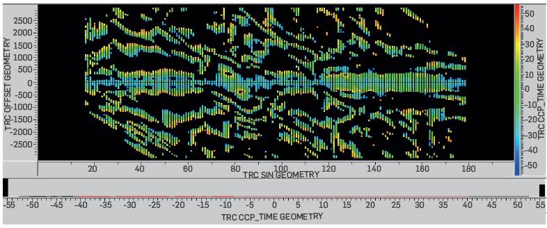
Figure 9 Cross-correlations. The horizontal axis represents the shots, the vertical axis the offsets, and the colors represent the value of the cross-correlation.
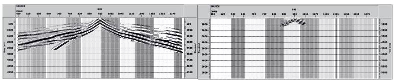
Figure 10 Application of intervals of offsets. Full residuals on the left, and residuals in the offset intervals for FWI on the right.
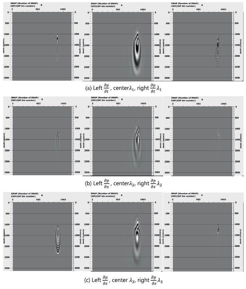
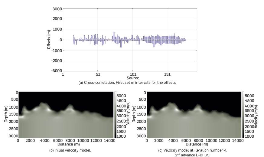
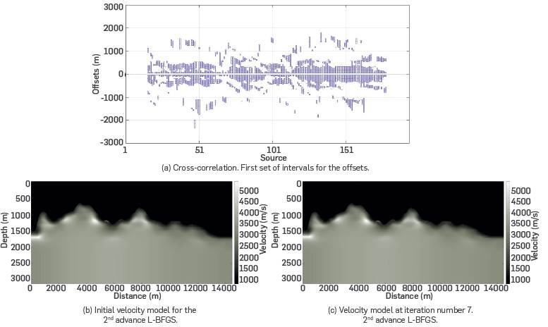
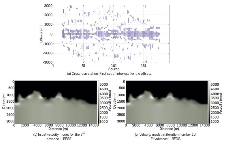
Figure 12 illustrates the cumulative gradient for the velocity model. Figure 13-a illustrates the velocity gradient after extracting the topographic information and removing the gradient information in the air layers. A topography mask is used for the removal of outliers in the more superficial layer (see Figure 13-b). An illumination mask is shown in Figure 13-c. Once the masks are applied to each gradient, the information provided by each vector shows the depth zone that will be updated, as it is shown in Figure 13-d. With the adjusted velocity and density gradients, the first update of the physical parameters is performed (see Figure 14). For quality control, it is verified that the cost function decreases as the iterations increases. Figure 14-a shows the cross-correlations for one set of offsets. Figure 14-b shows the initial velocity, and Figure 14-c shows two updates using the L-BFGS method. Figure 15-a shows the cross-correlations when two sets of offsets are selected. Figure 15-b shows the initial velocity (velocity model 4), and Figure 15-c shows two updates using the L-BFGS method. Figure 16-a shows the cross-correlations when the third set of offsets is used. Figure 16-b shows the initial velocity (velocity model 7), and Figure 16-c shows two updates using the L-BFGS method. In all iterations, the cost function decreases, and the first velocity update uses the steepest descent method.
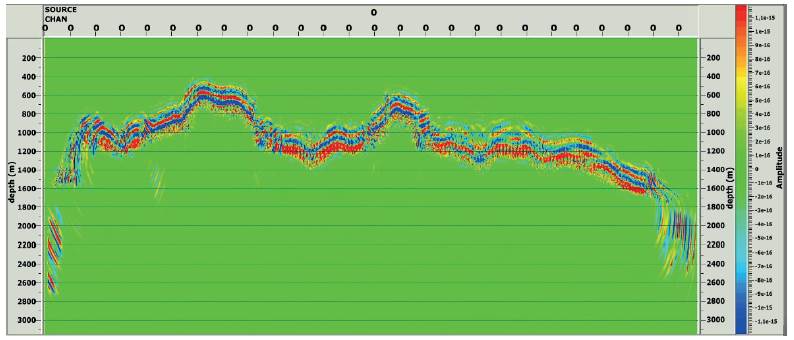
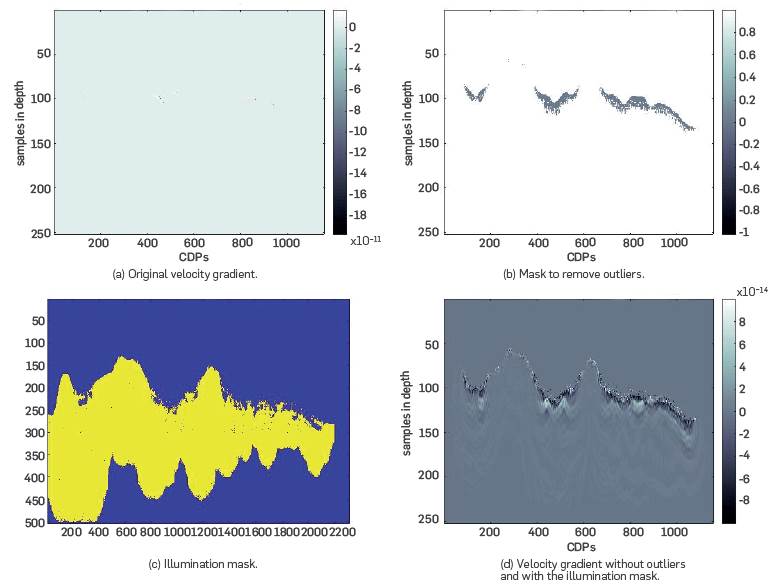
Figure 13 Application of the removal mask for the outliers and the illumination mask for the velocity gradient.
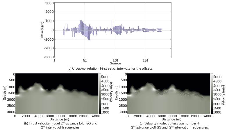
Finally, a new frequency content is selected to include more information in the estimation of the velocity and density models. Using Equations (3) and (4) with vmin = 777,111 m/s and vmax = 5.427,3 m/s, the discretization parameters chosen are Δt = 0,6 ms, Δh = 6,25 m. The first iterations of the complete waveform inversion can include information of a frequency content up to 12,43Hz. Figure 17-a illustrates the cross-correlations with the new residuals, starting from the velocity model 10. Figure 17-b shows the initial velocity, and Figure 17-c shows two updates using the L-BFGS method. At all iterations, the cost function decreases. The stopping criterion shows that the change in the cost function is no longer significant, and the inversion stops.
■ CONCLUSIONS AND DISCUSSION
All experiments were tested using an 8-core Intel (R) Core (TM) i7-4790 processor with 16GB of RAM, with a clock frequency of 3,6GHz. One single iteration of FWI for the Dip 2D line in the first range of frequency spent 32,33 hours, and for the second range of frequency, it spent 64,33 hours. In terms of memory capacity, the memory resources per 2D line, for the first frequency range, did not exceed 4GB, and for the second range, 8GB. This work showed that it is feasible to apply the methodology proposed for land data sets FWI on the low resolution 2D line using a workstation with intermediate hardware requirements.
For all the tests described in this article, the FWI uses the method of steepest descent in the first iteration, and L-BFGS for the next iterations until the stopping criteria is reached. It should be borne in mind that not all the information present in the traces can be used from the beginning. Therefore, the events recorded by geophones must be classified according to their content in frequency, offset, amplitude, phase, and wave type (reflections, refractions, multiples). Thus, the pre-conditioning steps that select only the data to be used, and correct the time-lags between the modeled and observed data is crucial before applying FWI.
As a conclusion, the methodology studied in this work shows the effectivity of FWI applied to land data sets, despite the challenges of the method. The final velocity model built with FWI shows an uplift of the velocities in the areas with high elevations, and a down lift of the velocities in the foothill areas where there is accumulation of sediments that forms the alluvial soil. The next step in FWI for land data sets is to include advanced elastic models so that more events can be considered during the inversion process, and a better velocity estimation can be obtained.

