


 Inglês (pdf)
 Artigo em XML
 Referências do artigo
 Enviar este artigo por email
 Citado por SciELO
  Citado por Google
  Similares em
SciELO
Similares em
SciELO  Similares em Google
 Permalink
1. INTRODUCTION
The Economic European Community first started taking measures to reduce vehicle air pollution in 1970, and with new regulations, it has defined various test types, methods, and technical specifications for measuring exhaust gas emissions. Later, vehicle-borne air pollution legislation was introduced as the EURO emission standard in 1991, coming into force in July 1992 as EURO 1.
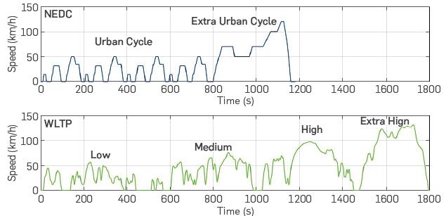
The New European Driving Cycle (NEDC) took its final form in 1997, as a standard driving cycle still relevant today. This driving cycle is an 11 km long cycle consisting of 4 urban cycles and an extra-urban cycle. The speed profile in the driving cycle is tracked exactly by the driver in the vehicle on the chassis dynamometer. Changes in the vehicle's speed, acceleration, and gear changes should be within specified tolerances. Before testing, the vehicle must be preconditioned in a 20-30 °C ambient temperature for at least 6 hours to ensure that the coolant and engine oil are within these temperature range. Gases from the exhaust pipe are collected in one or more bags by the constant volume sampling (CVS) method while the vehicle is running, and subsequently analyzed following a rigorous procedure. According to this cycle, emission amounts such as CO, NOx, HC, and particulate matter per kilometer (g/ km) are calculated to compare with EURO standards. NEDC cycle is a reference cycle used up to Euro 6 in Europe and some other countries [1 - 5].
The document containing fuel consumption values and emission values obtained from the NEDC cycle for each vehicle is publicly available, and it is used in the eco-label created for the users to opt for a vehicle. However, there are significant differences between fuel consumption and emission values obtained in real road conditions and homologation values. These differences are reported in many studies. Tzirakis et al. [6] compared a typical Athens cycle with the NEDC cycle and found a 56-79% increase in fuel consumption. The same trend of fuel consumption increase has been observed in CO2 emissions in their study. While NOx emissions increased by 300% on a g/km basis, a 132% increase was observed in CO emissions, and there was no change in HC emissions.
The differences between real road driving cycles and NEDC can translate into 12-30% more fuel consumption and 32.2-62.83% more real road cycles in NOx emissions [7].
Three vehicles with EURO 2, EURO 3, and EURO 4 were subjected to ECE and EUDC driving cycles on the chassis dynamometer and the results were compared to the Belgian MOL driving cycle [8]. A similar conclusion has been reached in this study. In this driving cycle, an increase between 15% and 25% in fuel consumption and CO2 emissions of EURO 3 and EURO 4 vehicles was observed. Significantly different results were also obtained for CO and NOx emissions.
In a study published by the European Commission Joint Research Center, the type approval certificate data were compared with real road data using fuel consumption values from various studies such as the Artemis project, ADAC (Allgemeiner Deutscher Automobil-Club) organization in Germany, automotive magazines [9]. It was determined, as a result of the study, that the fuel consumption values stated in the certification are 10-15% below the real values, and 12-20% less in diesel vehicles.
While a typical gasoline vehicle performs the NEDC cycle, it runs below 2500 rpm at 90% of the cycle, and spends 85% of its time to overcome the wheel power below 10 kW [10]. Hence, the engine/ vehicle is effectively tested in a small operating range. Therefore, the NEDC cycle is defined as a low-load driving cycle that only allows for effective testing in a narrow working range [11]. The cycle does not reflect the actual driving conditions: accelerations are very soft, idling times are high, and situations with constant speed are more than necessary.
Based on the foregoing, a search for a driving cycle that could replace the NEDC started recently. Also, the diesel emission scandal arisen in 2015 resulted in pressure on the new cycle. The WLTP (Worldwide Harmonised Light Vehicles Test Procedure) and the WLTC (Worldwide Harmonized Light vehicles Test Cycles) are global accepted standards developed to determine pollutant levels, CO2 emissions, and fuel consumption of classic and hybrid electric vehicles, and the ranges of purely electric vehicles. This new protocol was developed and launched in 2015 by the United Nations Economic Commission for Europe (UNECE) to achieve fuel consumption and emission values closer to real road driving conditions in laboratory tests. Thus, the WLTP has been replaced by the NEDC cycle as the European vehicle approval procedure [12,13]. The new standard cycle is designed to better represent today's real driving conditions. To achieve this goal, a speed profile with longer, more dynamic, faster acceleration, and short braking times was developed in WLTP vs. NEDC. Thus, a driving cycle of 23.25 km in length was achieved, with an average speed of 46.5 km/h, and a maximum speed of 131.3 km/h.
The main differences between the old NEDC and the new WLTP test, or the basic features of WLTP are:
Average and maximum speeds are higher in WLTP;
WLTP consists of a wider range of driving conditions such as urban, highway, suburban;
WLTP has a longer distance;
It has a higher average and maximum driving power;
Steep accelerations and decelerations;
Allows testing optional equipment individually;
Offers hot and cold engine operating conditions.
In this study, the vehicle mathematical model was created in a MATLAB program using vehicle longitudinal motion equations for a light commercial vehicle with a diesel engine. The speed profiles of NEDC and WLTP cycles are defined in the model, and the fuel consumption, CO2 emission values, and total energy values required for each cycle are calculated. Further, the recoverable energy potentials of the cycles have been revealed. The results were achieved after considering the fuel cut-off and start-stop strategies proposed in the modelling to improve fuel economy. Thus, it proposes a comparison of the WLTP cycle that has just been introduced and the classical NEDC cycle for a vehicle.
MATHEMATICAL MODEL OF THE VEHICLE
There are two approaches as a forward and backward vehicle model for modelling of a vehicle. In the forward vehicle models, the input signal is a force applied on the accelerator or brake pedal. In the backward vehicle model, the input is a driving cycle. The required power and torque at wheels are calculated according to the defined driving cycle. Then, they propagated back to the power source (internal Combustion Engine/ICE) through the drivetrain. This approach is suitable for determining the power and energy required in a driving cycle [14].
This paper compared the fuel consumption and energy need of the vehicle considering the NEDC and WLTP driving cycles, which are the most known. The backward vehicle model was created in MATLAB. The driving cycles were defined as a look-up table, and imported to the model. In the first column of the lookup table, time was defined at one-second intervals; vehicle speed and gear position were also defined in the second and third columns. After calculating the traction force required to overcome resistance forces, the engine effective power was calculated, taking into account the efficiency of the driveline. The parameters used in this study are shown in Table 1. The vehicle considered is a light commercial vehicle with a 1.3 lit diesel engine.
Figure 1 shows the flow chart of the fuel consumption model. Instantaneous fuel consumption was calculated by interpolation from a specific fuel consumption map of the engine, and total fuel consumption, traction energy, and braking energy were calculated for both driving cycles.
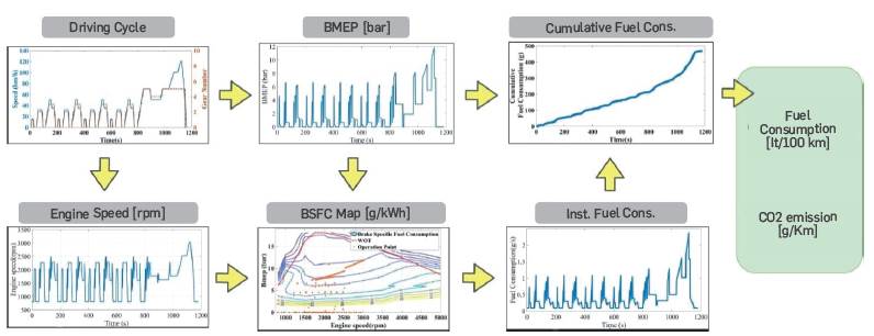
In the brake specific fuel consumption (bsfc) map of the engine, the horizontal axis is engine revolution (rpm), and the vertical axis is brake mean effective pressure (bmep). To read instantaneous fuel consumption on the map, the current speed and the bmep value of the engine must be known. Engine speed is calculated depending on the wheel speed and gear ratio (Equation 1). The bmep is calculated using the engine's revolution and effective power, as shown in Equation 2. The engine effective power is also calculated as shown in Equation 3. All the following equations are taken from [15].
where v is the wheel speed, R w is the wheel radius, i g and i d are gear ratios of the gearbox and differential, respectively
Table 1 Parameters used in the model
where P e is the effective power of the engine (kW), n is engine revolution (rpm), V H is engine displacement (lt). The effective power of the engine can be calculated using traction force (F traction ) and motor angular velocity (ω) from Equation 3.
where T e and η t are engine torque (Nm) and efficiency of driveUne, "espectively. The traction force at wheels is calculated with Equation 4. Terms in the equation are rolling resistance, slope resistance, aerodynamic resistance, and inertial force, respectively. The sum of these forces is the given traction force at wheels. The traction force was calculated for a road without slope and wind.
where Ftraction is traction force at wheels (N), µ is the rolling resistance coefficient, m v is vehicle weight (kg), g is the gravitational acceleration (m/s2), cris the slope angle of the road, p is the density of air (kg/m2), Ctf is drag coefficient, is the frontal area (m2), v and v w are vehicle and wind speed, respectively (m/s), meq is the equivalent mass of the vehicle (kg), a is acceleration (m/s2). The rotating parts such as crankshaft, transmission primary and seconder shafts, differential, and wheels, also affect vehicle performance while the vehicle's is moving. Therefore, an equivalent mass (Equation 5) s calculated by reducing the inertia forces of these parts to the wheel axis.

where m v is vehicle mass. J e , J p , J s , J d , and Jware rotational inertias of the engine, the primary shaft of the gearbox, the secondary shaft of the gearbox, differential, and wheel, respectively. i g is the ratio of the gearbox, and i d is the ratio of the final drive, and R w is also the "adius of the tire.
Based on the above equations, after calculating the engine speec and bmep depending on the driving cycle, the instantaneous fuel consumption (m) can be read from the engine map. The cumulative fuel consumption is also calculated as shown below.
where V fuel is the amount of fuel consumed in 100 km on It basis, m is instantaneous fuel consumption (kg/h), ρfuel is the density of fuel (kg/It), and D is the distance of the driving cycle (km). During the driving cycle, the amount of CO2 released can be obtained from Equation 7. This equation is given for diesel fuel.
Traction energy and braking energy are calculated by interpolating the engine power as shown in Equation 8 and 9, respectively.
where E traction and E braking are traction energy and braking energy, respectively. P e,a >0 engine power at acceleration, Pe,0<0 is the engine power at deceleration.
COMPARISON OF NEDC AND WLTP DRIVING CYCLES
To evaluate the performance criteria of vehicles such as fuel consumption and emissions, different driving cycles are developed and standardized. One of the most widely used of these cycles is NEDC. NEDC was developed in 1980. It consists of an urban cycle rerpeated four times, followed by an extra-urban cycle. While the urban cycle is characterized by low speed and low engine load, the extra-urban driving cycle is characterized by a relatively higher speed and more aggressive driving. Because it is simple and has several stable driving modes, NEDC is a repeatable driving cycle. However, it does not represent real driving current performance, so it does not reflect real fuel consumption values and emissions [16]. In 2009, a project was launched by the United Nations Economic Commission for Europe (UNECE) to develop a harmonized driving cycle and test procedure [17]. Within this paper's scope, the Worldwide Harmonised Light Vehicle Test Procedure (WLTP), created by collecting real driving data worldwide, with a more realistic speed profile, was developed and implemented in 2017 [18]. The WLTP driving cycle consists in four different speed profiles, i.e. low, medium, high, and extra high. This newly developed driving cycle is more dynamic and longer than NEDC. The comparison of NEDC and WLTP cycles is shown in Figure 2 and Table 2.
Table 2 Basic parameters of NEDC and WLTP
| Parameter | NEDC | WLTP |
|---|---|---|
| Time(s) | 1180 | 1800 |
| Distance (km) | 11.03 | 23.27 |
| Maximum speed (km/h) | 120 | 131.3 |
| Average speed (km/h) | 33.6 | 46.5 |
| Maximum acceleration (m/s2) | 1.04 | 1.67 |
| Mean acceleration (m/s2) | 0.59 | 0.41 |
| Minimum deceleration (m/s2) | -1.39 | -1.50 |
| Mean deceleration (m/s2) | -0.82 | -0.45 |
| Constant driving percentage (%) | 40.3 | 3.7 |
| Stop duration percentage (%) | 23.7 | 12.6 |
| Percentage of acceleration (%) | 20.9 | 43.8 |
| Percentage of deceleration (%) | 15.1 | 39.9 |
A vehicle completes only 13% of the WLTP cycle at idle speed, 4% at a constant speed, and 84% of the cycle in accelerated motion. In the NEDC cycle, the vehicle completes the cycle by moving 36% of the cycle with accelerated motion, 24% at idle speed, and 40% with constant speed [17].
The differences between NEDC and WLTP are not only duration and speed profiles. Another significant difference is vehicle test masses, UNECE Nu.83 regulation is used to determine NEDC vehicle test mass, and UNECE GTR Nu.15 regulation is used to determine WLTP vehicle test mass [19]. In chassis dynamometer tests performed according to the NEDC cycle, the vehicle is tested only with standard equipment. The test mass is the sum of the vehicle's curb weight and driver weight. In the WLTP cycle, tests must be conducted on a fully equipped vehicle, including all equipment that is not included in the standard vehicle but can be added depending on the driver's request [20], and there are two different test mass definitions according to the "optional equipment" weight: Low Test Mass (TML) and High Test Mass (TMH). The difference is that optional equipment weight at high test mass is included, while optional equipment weight at Low test mass is not included. High Test Mass (TMH) is mainly used in WLTP tests. These masses can be obtained from the sum of the components in Equations 10 and 11 [19].
Here, mr consists of vehicle mass equipped with standard equipment, driver's weight, and the fuel tank weight of 90% full; m equip , is the weight of optional equipment. It is difficult to determine the equipment's weight accurately, but Ligterink et al. [19] says that the optional equipment weight could be considered between 50 and 225 kg. Also, m max is the maximum weight of the vehicle. In this study, the test weight for the WLTP cycle was calculated according to TMH, and the optional equipment weight was accepted as 200 kg.
3. MODEL VALIDATION
For model verification, the results of the model and test values of the vehicle were compared in Table 3. The differences between modelling and test values are acceptable. The described model is suitable for providing reliable values of vehicle fuel consumption, even when cold start cycles are considered. The main uncertainty stems from the "driver effect", which is an uncertainty also during experimental tests.
4. RESULTS
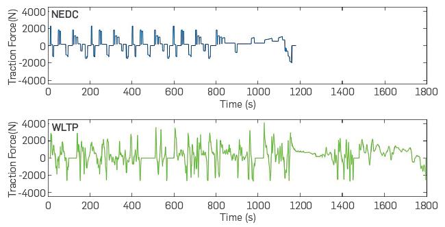
The traction force graphs required by the vehicle during the NEDC and WLTP cycles are shown in Figure 3. It was mentioned in Section 2 that the traction force applied from the wheels for the movement of the vehicle varies depending on the resistance forces and the inertia force of the vehicle. The test mass used in the WLTP cycle is higher than the mass in the NEDC cycle. Therefore, this affects the rolling resistance and the inertia of the vehicle directle. Thus, it is observed that the maximum traction force values in the acceleration and deceleration in the graphics are higher in WLTP. In the last phase of the WLTP cycle, the inertia is lower as the vehicle moves with low accelerations in the 5th gear. Therefore, lower traction force values were obtained. While the highest traction force required by the vehicle in the NEDC cycle is 2268.3 N, it can go up to 4091.6 N in the WLTP cycle.
When the Instantaneous traction power values of the vehicle during both cycles are analyzed, it is observed that the highest values are obtained in the extra high phase region of WLTP and the extra-urban driving cycle of NEDC (Figure 4). As with the traction force graph, the maximum traction power values in the WLTP cycle are higher than in the NEDC cycle, as it travels at relatively higher speeds. While the highest traction power required by the vehicle in the NEDC cycle is 35.31 kW, it can go up to 51.3 kW in the WLTP cycle.
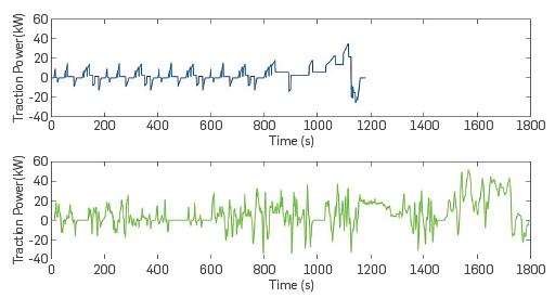
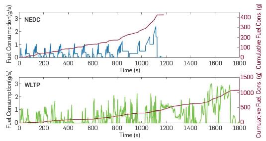
Figure 5 shows Instantaneous fuel consumptions. Since the fuel cutoff and start-stop strategies are considered, fuel consumption Is zero when the vehicle speed is zero (start-stop strategy), the engine speed is over 1000 rpm, and the accelerator pedal released (fuel cut-off strategy). As expected, instantaneous fuel consumption Is higher In regions with high traction power. The highest value of instantaneous fuel consumption Is 2.4 g/s in NEDC and is 3.0 g/s in WLTP. Also, the cumulative fuel consumption for both cycles is that shown in Figure 5. During the NEDC cycle, 423.22 g of fuel was consumed and 1070.8 g of fuel was consumed during the WLTP cycle. These fuel consumption values are obtained in hot engine conditions.
In the energy graph In Figure 6, the blue-colored regions show the energy values at positive acceleration and constant speed points. The red-colored regions show the energy values during braking. Regenerative braking systems recover the part of the braking energy In electric vehicles, but this energy is lost as friction and heat In conventional vehicles. Nevertheless, even in some classic vehicles, braking energy can be used to charge the battery. In these vehicles with a smart charging system, the alternator Is operated with braking energy and it benefits from this energy.
The total amount of energy required during the cycle was 6.21 MJ in the NEDC cycle and 18.43 M J in the WLTP cycle. In Table 4, all values are high for the WLTP cycle. This is because the WLTP cycle runs at higher speeds, and the test mass In WLTP Is heavier than In the NEDC. The expected result Is that the energy and CO2 emission values obtained will be higher In the WLTP cycle due to the different cycle distances. Hence, to make a more accurate comparison, the energy values are given in MJ/km In the table.
CONCLUSIONS
In this study, the vehicle mathematical model was created in a MATLAB program for a light commercial vehicle with diesel engine, and then fuel consumption, CO2 emission values, and energy need were calculated for the NEDC and WLTP cycles. The findings obtained at the end of the study can be summarized as follows.
When the traction energies of the cycles are compared 45% more energy Is consumed in the WLTP cycle relatively to the NEDC cycle.
81% of the total energy In the WLTP cycle is used for traction, while the remaining 19% Is spent for braking. In the NEDC cycle, 78% of the energy is used for traction and 22% for braking
When the average energy values are compared, the vehicle needs to spend 45% more energy than the NEDC cycle in the WLTP cycle. When the average braking energy values are compared, an increase of 25% is observed.
Braking energy In ICE vehicles can be recovered by using mechanical KERS (Kinetic Energy Recovery System) based on the vehicle's Inertia. The WLTP cycle provides more advantages in energy recovery during braking due to Inertia forces and higher braking energy.
CO2 emission of a diesel vehicle with active fuel cut-off and start-stop strategies is 11% higher In the WLTP cycle. Although the total emission amounts are higher In the WLTP cycle, since the distance is longer, the effect of cold start on CO2 emissions in the WLTP cycle Is less than In the NEDC cycle.
In recent years, tests to measure the fuel consumption and emissions of vehicles in real road conditions have become as important as laboratory tests. There are some difficulties such as the fact that RDE (Real Driving Emissions) tests are more comprehensive and take longer than laboratory tests, the risks that may be encountered in real road conditions while performing the test, and the Inability to test in difficult road and weather conditions, plus the waste of effort and time in possible test cancellations. Presumably, in the future, representation of real road tests under Laboratory conditions can be considered. Thus, although the WLTP test does not meet the values in real road conditions, it is relevant in terms of giving values closer to it, allowing for a correlation between laboratory and real road tests.
Test initial conditions are similar for both cycles, but in the WLTP cycle, the vehicle test mass is heavier, and road loads are more realistic. The vehicle travels at higher speeds, and the constant speed movement time accounts for only 3% of the entire cycle. This rate is much lower compared to the NEDC cycle. Therefore, the WLTP cycle provides a more dynamic speed profile, closer to real traffic conditions. Therefore, it renders more realistic and accurate results for type approval tests.

