English (pdf)
 Article in xml format
 Article references
 Send this article by e-mail
 Cited by SciELO
  Cited by Google
  Similars in
SciELO
Similars in
SciELO  Similars in Google
 Permalink
1. INTRODUCTION
The increase in the recovery factor of heavy crude oil fields depends mainly on achieving a decrease in its viscosity and favoring its displacement to the surface. Thus, the most widely used recovery method worldwide is steam injection. This technique allows heat to be transferred to the oil, reducing its viscosity, and modifying the capillary number, favoring its displacement. Traditional heat recovery methods that rely on steam or hot water injection, such as Steam Assisted Gravity Drainage (SAGD), Cyclic Steam Stimulation (CSS), and steam injection, have amassed substantial knowledge in this domain. Nevertheless, these approaches may encounter economic and environmental challenges given the considerable quantities of steam needed, and the reliance on extensive natural gas combustion, which is an Unsustainable situation due to CO2 emissions (Sivakumar et al., 2020). In terms of representing the physical phenomenon through modelling, the capacity of the electric field to induce polarization in the material and the resistance of this polarization to extremely rapid changes in the electric field result in various physical processes implied in the radio frequency (RF) heating of reservoirs. Recently, there has been interest in EM heating to overcome these challenges, which have inhibited steam-based recovery. The primary purpose of the electromagnetic heating system is to enhance the oil's mobility by decreasing its viscosity, achieved by heating the reservoirs through the conversion of electromagnetic fields into thermal energy (Sahni et al., 2000), (Bogdanov et al., 2011).
While RF heating processes are commonly used, modelling the complex interactions among oil, water, rock matrix, and RF antennas lead to significant challenges. Moreover, the availability of electromagnetic simulation tools specifically tailored for such scenarios is limited, thereby providing an opportunity to propose a novel methodology for modelling electromagnetic heating. Despite the extensive study of this radiofrequency recovery technique over the years, the use of numerical simulation techniques within the reservoir industry for electromagnetic heating in heavy oil reservoirs connected to bottom aquifers has been constrained. This paper presents a comprehensive time-domain combined finite-difference numerical model that integrates electromagnetic and heat transfer processes. The model accounts for the fractions and saturation of reservoir phases, as well as the temperature-dependent electrical and thermal properties of the reservoir phases. This allows for determining the required energy in kWh and its influence on the antenna power, as well as the thermal and electrical properties of a medium in the presence of aquifers.
2. THEORICAL FRAMEWORK
SOLUTION OF MAXWELL'S EQUATIONS IN DIELECTRIC MEDIA WITH LOSSES
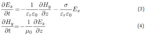
Maxwell's equations are a concise way of establishing the fundamentals of electricity and magnetism. We use it as a starting point to simulate advanced features of electrical and magnetic phenomena, in the form of differential equations. To simulate electromagnetic propagation, we specify the relative dielectric constant because a material's response to an applied electric field depends on its permittivity εr(ω) = ε (ω))/ε0 where ε (ω) is the absolute permittivity, and which depends on the frequency of EM wave propagation in the medium. Now, for media such as heavy crude, there is a loss term associated with the conductivity that gives rise to energy attenuation and its heating effect on the reservoir. We can model the EM propagation of the wave fields (E,H) for media with conductivity-related loss using the following equations:
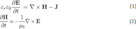
where the electric current density is denoted by J = σE. Systems with symmetry such as rectangular, cylindrical, and spherical systems are one-dimensional when the electric field, or the temperature in the body is only a function of distance, and independent of azimuthal angle or axial distance. Within the context of electromagnetic heating of heavy oil, modelling assumes a crucial role as an indispensable aspect of the process, demanding a careful selection of appropriate symmetry. It involves creating computer simulations or mathematical models to understand and predict the behavior of the system.
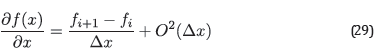
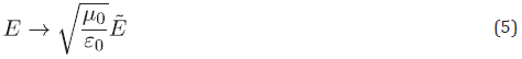
In these cases, the differential equations are simplified, obtaining a simple solution. In one dimension, equations (1) and (2) can be expressed as:
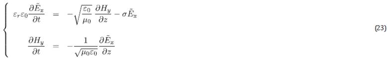
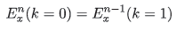
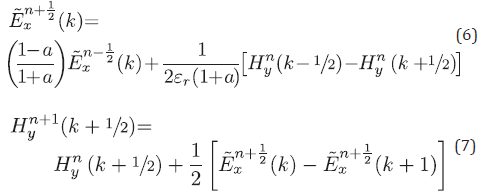
These equations model EM propagation in the z direction with the electric field oriented in the x direction and the magnetic field in y. Now, since Equations (3) and (4) are similar, but E0 and Μ0 differ by several orders of magnitude, Ex and Hy also differ in magnitude. A normalization is possible by changing the following variables:
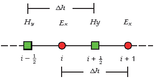
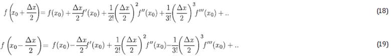
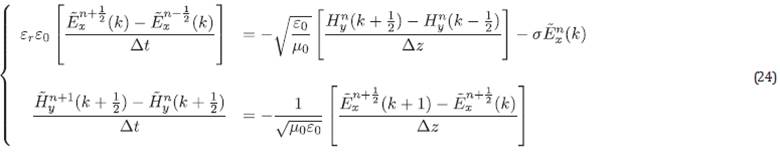
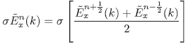
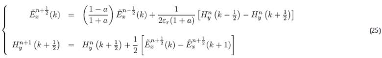
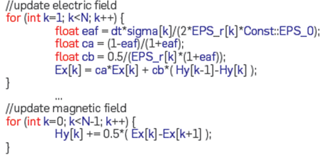
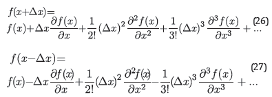
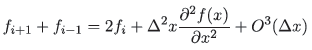
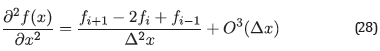
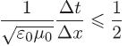
Using the centered and staggering finite difference approximation (FDTD Finite Difference Time Domain) for both the spatial and temporal derivatives, according to Taflove & Hagness (2005) and Sullivan (2013), we have that:
where
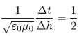
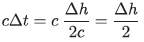
 with a numerical stability
=
-.
with a numerical stability
=
-.  condition
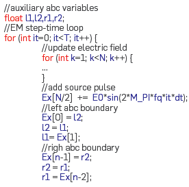
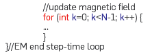
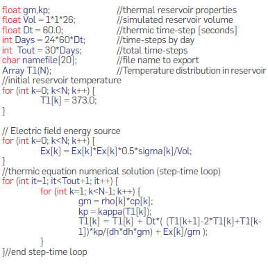
The fields Ex and Hy are computed in the discrete equations (6) and (7) at the k-th node of the mesh, and the time-step computation is denoted by n + 1, meaning that the times are staggered between fields. With these two expressions, we calculate the EM power generated for each point in space. In the appendix, there is a more detailed discretization using the FDTD technique and its coding in C++ language.
The movement of charged particles is caused by the introduction of an electric field in a dielectric material. Charges are moved out of their equilibrium positions, creating induced dipoles that react to the applied electric field. By opposing the dipoles in the medium, a time-varying EM field of significant amplitude causes a dissipation of power inside the material, which manifests as a rise in temperature (Meredith, 1993), (Bogdanov et al., 2011). To tackle power absorption issues in EM propagation, in both radio-frequency and microwave, lossy medium modelling is used.
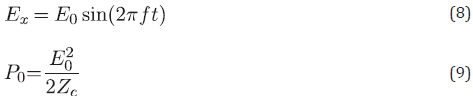
Conduction heat transfer is the main process model based on EM heating. To carry out the simulation of the reservoir heating process, a sinusoidal radio frequency source is selected. The expression associated with the time-varying electric field generated by such source is given as:
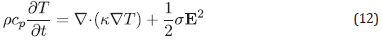
To generate the electric field E0 the power P0[W ] per unit area is delivered to this region of interest as a fraction of the total power, and it is set with reference to nominal values from 5[kW ] to 30[kW]. Equation (9) shows the relationship between the delivered power and the incident electric field amplitude, where Zc is the intrinsic reservoir impedance that, for practical purposes, we will take as 1.
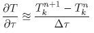
HOW TO CALCULATE THERMAL VARIATION
As a heat source, the coupling term between the equations for the EM field and the heat flux can be expressed as

The value of the effective electrical conductivity a* of the reservoir depends on the EM wave propagation frequency, temperature, and fluid composition (Bogdanov et al., 2011). It is a complex type value that accounts for the medium's dielectric and conductivity properties. The increase in temperature can be calculated from the following equation as a porous media saturated with any fluid absorbs EM radiation.

This means that the source of energy generated by the electric field must be included in the solution of the temperature distribution. Then, the field energy intensity is associated with the square of the electric field amplitude E2. The following figures, 5-a and 5-b, show the value of the electric field and its energy for two different power values at 400 [MHz]. It is observed that a higher power in the antenna (10[KW]) represents a higher electric field amplitude and, in turn, a higher energy distributed inside the reservoir.
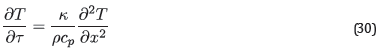
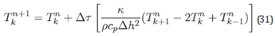
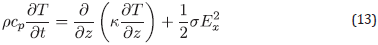
The temperature distribution is obtained from the EM heat calculated from equation (11), the following numerical model describes the electromagnetic and thermal problem in a coupled manner without considering the motion of production fluids and is governed only by the thermal energy conservation equation.
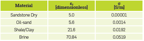
or, in equivalent manner, in the z-direction for a reservoir column 1x1x26 [m3]
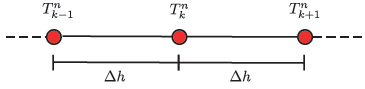
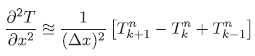
The explicit finite difference discretization (see appendix for further description) would be:
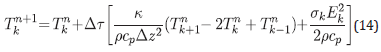
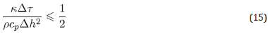
The Δx variable can be represented in terms of seconds, hours, or days. The equation (14) is numerically stable if it meets:
Heat generation is a volumetric phenomenon and it occurs in the medium where EM waves propagate. That is, heat generation in a medium is usually specified per unit volume and is represented by  which is given in [W/m3] units (Cengel & Ghajar, 2021). When the variation of heat generation with respect to position is known, the total rate of heat energy generation for the volume V can be determined as shown below:
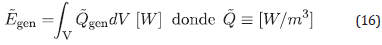
Therefore, the value of the heat generating source must be considered in the expressions (12), (13) and (14) as:
3. METHODOLOGY
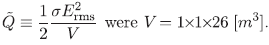
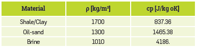
The electromagnetic field computation simulates the behavior of the electromagnetic field with the electrical properties of the conductive materials. These simulations help determine the distribution of the magnetic field and the induced electric currents within the oil reservoir. Table (1) presents the relevant factors considered in the modeling of electromagnetic heating of heavy oil reservoir material. These factors of reservoir properties play a crucial role in determining how the material reacts to the electromagnetic fields applied during the process (Kasevich et al., 1997), (Daniels, 2004).
Figures (1) and (2) show modeled values for EM propagation in a reservoir made up of two materials, with each other's dielectric and conductive properties based on table (1). A reservoir model with Sandstone Dry and Clay/Shale material and other with Sandstone Dry and Oil- Sand.
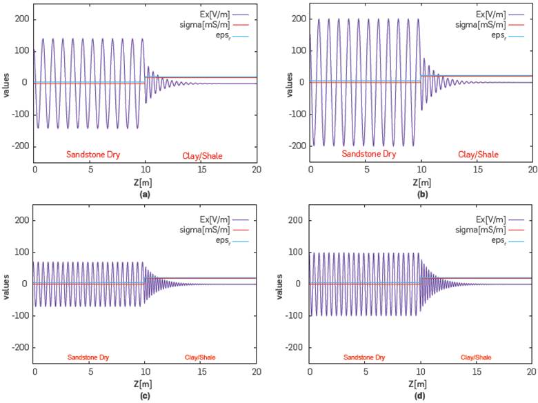
Figure 1 Propagation of an electric wave field in the depth direction z[m] for a porous media with clay/shale material. (a) 150[MHz] and 5[kW] of power, (b) 150[MHz] and 10[kW] of power, (c) 300[MHz] and 5[kW] of power, (d) 300[MHz] and 10[kW] of power.
In order to determine the time step At in the EM modelling, the EM field frequencies are taken in n parts per oscillation cycle (Tcycle)
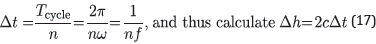
Figure (1) shows the evolution of the electric field Ex for a source or antenna located at z = 0[m]. Radio frequency is related to the number of oscillations of EM radiation per second. Generally, all frequency ranges from 3 kHz to 300 GHz are called radio frequencies. In general, RF are either transmitted by a material, absorbed, or reflected depending on the properties of the material. These waves are stimulated by the dielectric interaction for different values of field amplitude (antenna power) and frequency. Figure (1a) shows the propagation with a power of 5kW and 150MHz, figure (1b) 10kW and 150MHz, figure (1c) 5kW and 300MHz and figure (1d) with 10kW and 300MHz. An attenuation of the wave field on the right side is observed, represented by the clay/shale material. According to Table (1), this material has high values sr, a with respect to the material or medium Sandstone Dry. There is a strong change of oscillation amplitude with a resonance effect on the Sandstone zone. This same behavior can be observed in a brine-saturated medium, because the conductivity and dielectric material are high. In other words, the electromagnetic power is attenuated in a medium with higher electrical conductivity.
Table 2 Parameters modeling for a 150Hz EM field propagation. The values have been calculated for n = 70 parts of an oscillation cycle of the electric field.
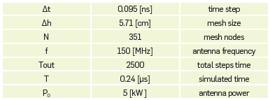
Figure 2 Propagation of an electric wave field in the depth direction z[m] for a porous media saturated with oil. (a) 150[MHz] and 5[kW] of power, (b) 150[MHz] and 10[kW] of power, (c) 300[MHz] and 5[kW] of power, (d) 300[MHz] and 10[kW] of power.
Figure (2) shows the transmission and reflection behavior of the EM wave for an Oil-Sand medium. The same numerical experiment was repeated with the antenna placed in a Sandstone-Dry material (z=0), but interacting with a slightly larger dielectric and conductive medium (see Table 1). In short, RF is transmitted, absorbed, or reflected depending on the properties of the material. It is interesting to note that in Oil-sand porous media, regardless of the value of the propagation frequency from 150 or 300 MHz, the value of the electric field amplitude plays an important role (Figure 2). In a highly conductive media such as Clay/Shale and Brine, high frequencies have higher attenuation despite the EM field amplitude (Figure 1).
We will now describe a simulated reservoir model in which RF waves will propagate through the formation to model EM heating. Figure (3) shows a modeled reservoir with a centrally located transmitting power antenna. This image showcases a simplified electromagnetic heating model for reservoirs exhibiting vertical heterogeneity. The model specifically represents a heavy oil reservoir connected to bottom aquifers, capturing the interaction and interdependence between the electromagnetic heating phenomenon and the geological formations that are characteristic of such reservoirs. The proposed simplified model serves to enhance the understanding of behavioral dynamics associated with electromagnetic heating within these reservoir configurations.
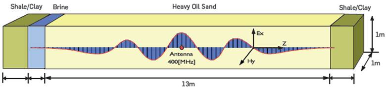
Figure 3 Proposed model of electromagnetic heating represented in a heavy oil reservoir connected to strong-bottom aquifers. The model is a pseudo-3D in 1D where its reservoir volume is 1x1xDepth.
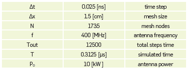
As characteristics of the simulation model, we have a volume of 1x1x26 [m3] with mesh size dh that depends on the EM wave propagation frequency, and based on the criteria of equation (17), the thickness of the reservoir sand is 13m, while in the upper and lower impermeable clays, it is 5m each. The heavy oil has been represented as monocomponent of API 14, and its dielectric properties are based on table (1). At the bottom of the sand, there is a brine-saturated zone, 20k ppm saline. Table (3) shows simulation parameters.
Table 3 Parameters modelling for a 400Hz EM field propagation. The values have been calculated for n = 100 parts of an oscillation cycle of the electric field.
From the antenna site towards the formation borders, it is noted that the EM field amplitude decreases (figure 4-a and 4-b). We chose the 300 MHz and 400 MHz frequencies as these are used in real-world technology demonstrations. We also have an abrupt attenuation of the EM field for the zone saturated with brine. This zone is demarcated by the red color lines, and it corresponds to high values of electrical conductivity with respect to the other reservoir rock materials. A similar attenuation behavior is shown for the brine zone in previous models with frequency values of 150 [MHz]. Now, as shown in both parts (a) and (b) of the figure, the variation of the field amplitude is also attenuated by the electric field in the seal zone of the reservoir, which is a zone of influence given the high electrical conductivity of this type of rock with respect to a sandstone.
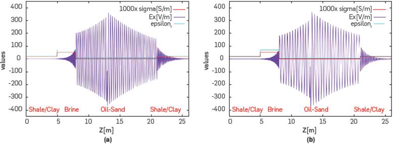
Figure 4 Electric field propagation at 400 [MHz] and 300 [MHz] images (a) and (b) respectively with 10 [kW] power. The electric field [V/m] is represented by the purple line and the electrical conductivity [S/m] in the reservoir by the red line.
A high electrical conductivity, given by the water saturation of the formation, influences the electric field amplitude and the effects of EM wave propagation frequencies within the medium. These phenomena influence heating, as will be demonstrated with the incorporation of the thermal radiation model into the diffusion equation. Modeling can provide insights into factors such as heat distribution, energy efficiency, and the overall performance of the electromagnetic heating system.
4. RESULTS
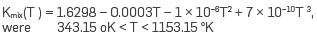
The EM heating modelling has considered estimating the temperature dependent thermal conductivity K = K(T) considering the mixing fractions for water+oil+rock. The following is an estimated polynomial relationship for the thermal conductivity based on these fractions.
In the 20[kW] case, the solution stabilized after 30 days of EM heating up to a maximum temperature of 170[oC] in the center of the reservoir. The solution stabilizes after multiple repetitions in comparable days, i.e. 3600 * 24 * 30[sec].
In contrast, the solution for the 30[kW] scenario stabilized after 30 days of EM heating to a maximum of 225 [oC] in the middle of the reservoir. This makes this type of heating considerably distinct from traditional heating, which has slower heating rates and depends on the material's thermal conductivity, temperature variations along the material's length, and convective currents. The heating of the reservoir and its temperature distribution are then significantly influenced by the dielectric characteristics of the rocks and the fluids they contain, as well as the antenna power.
There is a scaling factor that can vary the temperature distribution, which is associated with the volumetric heat (or energy) transfer. This suggests that it depends on the total thermal energy generation for a given volume of the reservoir to be modelled; in our case, we are evaluating a volume V = 1x1x26 [m3].
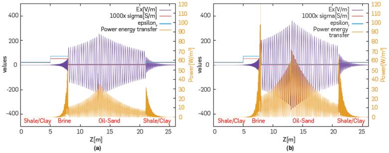
Figure 5 Figures (a) and (b) show the distribution of EM energy radiation at 400 MHz for 5 kW and 10 kW, respectively.
We can observe in the simulation that the presence of an aquifer (medium saturated with brine where εr = 70, σ = 0.0519[S/m]) affects the EM heating. We have modelled the temperature-dependent thermal conductivity. However, for a better description of the heating phenomenon.
The heating phenomenon, t medium density, heat capacity, conductivity and electrical permittivity must also vary with respect to temperature.
CONCLUSIONS
According to the FDTD simulation results, radiation from the RF heating passes through the material, transferring heat from the antenna position to the outside. Electromagnetic heating can be an effective oil reservoir stimulation approach and we identify zones where EM field amplitude values favor heating.
In reservoirs with oil sands, or exceptionally high viscosities, where the temperature influence on viscosity is relevant, electromagnetic heating could be used as a pre-heating method to establish preferential channels for steam injection. Steam injection performance would improve while minimizing heat losses, and the EM method can be combined to mitigate this, but there are few applications of electromagnetic heating to evaluate combined methods. This methodology allows for joint assessment because it can be implemented as a stand-alone tool. We present a numerical scheme that estimates temperature variations in the reservoir by electromagnetic absorption, based on the calculation of the radio frequency wavefield amplitude and radiation heat diffusion coupling that can be incorporated into industrial reservoir modeling software.
We include a comprehensive modeling study focused on the behavior of electromagnetic wave propagation within a reservoir containing heavy crude oil, coexisting with an aquifer, and considering the influence of their respective electrical and thermal properties. The thermal distribution within the reservoir is analyzed through diffusion over varying time frames, ranging from hours to days or weeks.
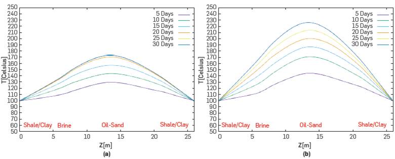
Figure 6 EM heating within the reservoir for various day intervals. Figure (a) shows the temperature distribution for a 20kW power and 400MHz antenna frequency. Figure (b) shows the temperature distribution for 30kW power with the same 400MHz antenna frequency. The horizontal line in the reservoir temperature distribution model represents the depth in meters.
This modeling approach allows us to precisely determine the required energy in kilowatt-hours (kWh) and its consequential impact on the radiating antenna's power in reservoirs that incorporate aquifers. Our research highlights the significant effect of water disruption on the heating dynamics within the reservoir.
To address this aspect, an alternative design is considered, incorporating a secondary antenna positioned within the reservoir. Through this approach, we observe promising results in enhancing thermal energy distribution, particularly if there is a significant presence of aquifers. These findings have material implications for optimizing electromagnetic heating strategies in heavy oil reservoirs, considering the intricate influence of underlying aquifers.
Depending on the reservoir and fluid characteristics, different types of electromagnetic heating can be used, including microwave and radio frequency based on the frequency band it operates in, which plays a key role in reservoir heating. It is necessary to have a solid understanding of how the electrical characteristics of reservoir dielectric materials change with temperature, pressure, and fluids. It is recommended to conduct laboratory analysis of the dielectric properties of rock samples saturated with different fluids at different temperatures and pressures for a better fit in reservoir modeling parameters for heating. It is also recommended to evaluate 2D and 3D simulations by addressing the resolution of initial value and boundary problems through the integration of coupled physical models using finite elements. This approach is particularly suitable given the complex nature and heterogeneity of the reservoir, which cannot be adequately addressed only by symmetry considerations.