


 English (pdf)
 Article in xml format
 Article references
 Send this article by e-mail
 Cited by SciELO
  Cited by Google
  Similars in
SciELO
Similars in
SciELO  Similars in Google
 Permalink
Introduction
A fundamental task in evolutionary multiobjective optimization (EMO) consists in the explicit computation of the set of solutions (known as the Pareto set) and their images (the Pareto front) corresponding to the problem of simultaneous optimization of multiple objective functions, or multiobjective optimization problem (MOP), for short. It is an important fact (see, e.g. [7]) that every non-trivial MOP admits more than one solution, i.e., there is no single point that simultaneously optimizes all the objective functions. A solution is called Pareto optimal if there is no objective function that can be improved without degrading the rest. Even though the Pareto set P of a MOP, consisting of the set of all optimal solutions, turns out to be a compact subset of Rn in common situations, generally it cannot be calculated in a purely analytical way, and the use of numerical algorithms becomes essential.
It is often desirable (and even necessary) to approximate P with a subset A⊂ℝn, called archive, that resembles P and its properties as closely as possible. Archives are usually assumed to consist of a finite number of points that can be numerically found, and EMO algorithms are an important tool employed for achieving that aim. To measure their accuracy, the distance between an outcome archive A and the original Pareto set P should be defined in an appropriate sense, but several inequivalent notions of distance can be considered, and their values are not necessarily attained in a unique manner. This means that the set of candidate approximations is usually not unique.
A readily available notion of distance between sets that can be used in this setting is the Hausdorff distance (see, e.g. [4]), but due to its definition, it allows for undesirable ambiguities, and heavily punishes single outlier solutions. Alternative performance indicators have been introduced in the literature (see, e.g. [10]) and among them, the averaged Hausdorff distance Δ p was recently proposed in [9] by modifying the well-known generational (GD) and inverted generational (IGD) indicators, in such a way that their values correspond to useful averages. As a result, Δ p does not punish individual but collective behavior, fixing some drawbacks of the standard Hausdorff distance. Other properties of Δ p have been investigated in the literature, for example, from the theoretical side that we are interested here, explicit analytical calculations of optimal archives with Δ p for particular Pareto fronts have been obtained in [8].
In this work, we establish conditions ensuring the Pareto compliance of the GD p and IGD p indicators by means of mathematical criteria involving the behavior of candidate solutions, and summarize at the end the consequences for the compliance of the averaged Hausdorff distance. The proofs require only simple properties of Δ p (or the intermediate GD p and IGD p ) derived from their definitions, which will be recalled in the section on preliminaries.
It is expected that these criteria for compliance with Pareto optimality can help to elucidate advantages and possible drawbacks of Δ p as a performance indicator for the evaluation of MOEAs. This is a necessary step in view of the possibility to modify and generalize the averaged Hausdorff distance with the purpose of enhancing its usefulness for applications. In fact, promising generalizations are already appearing in the literature for both, the cases of finite and continuous approximations (see [12] and [1], respectively). Further work in this direction requires a detailed understanding of the behavior of the original p -indicators, and the treatment presented here reveals also relevant aspects that should be considered.
This paper is organized as follows: In Section 2, we briefly present the background and notation required for the understanding of the rest of the manuscript. The core of this work appears in Section 3, where different criteria for the Pareto compliance of all the indicators, GDp, IGDp and Δ p are provided, including complete proofs, particular examples and important observations. Finally, conclusions and perspectives for future research are pointed out in Section 4.
Preliminaries
Throughout the document we will employ the abbreviations ℝ* = ℝ \ {0} and ℝ+: = [0, ∞) whenever necessary.
Multiobjective Optimization
Given a decision space X ⊂ ℝn and a vector valued function F: X ⊂ ℝn → ℝk defined on it, a multiobjective optimization problem consists in the simultaneous minimization of its k components f 1, ..., f k . A solution is called Pareto-optimal when the elements of the image, or objective space, Y = F(X) are non-dominated in the sense of Pareto [7]. This notion is defined in terms of a partial order relation that in this context and for our purposes can be introduced directly on X ⊂ ℝn, as follows.
Definition 2.1. For x, x' ∈ X the Pareto partial order ≤ associated to F is defined by
x ≤ x' if and only if f (x) f (x') for all i = 1,...,k.
Additionally:
An element x ∈ X is said to be dominated by x' ∈ X and denoted x' < x, if x'≤ x and f (x) ≠ f (x').
An element x ∈ X is dominated by A ⊂ X, written A ≤ x, if there exists some α ∈ A such that α ≤ x, otherwise it is said to be non-dominated by it, A
 x.
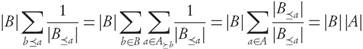
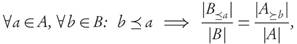
x.A subset A ⊂ X is dominated by a subset B ⊂ X, and written B ≤ A, if for every α ∈ A there exist some b ∈ B such that b ≤ a. If this is not the case A is said to be non-dominated by B and denoted B
 A.
A.An element x ∈ X is called Pareto-optimal if it is non-dominated,
 , and the set P, of all Pareto-optimal points is called the Pareto set.
The Pareto front is defined as the image F (P) of the Pareto set P ⊂ X.
Throughout the rest of this document we make use of the following handy abbreviations
Notation 2.2. For A, B ⊂ X and an arbitrary x ∈ X we define the subsets:
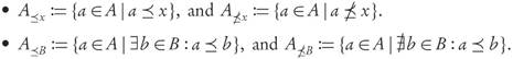
Clearly for any x ∈ X, or any B ⊂ X we have that: 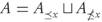 , and
, and  , where U denotes a disjoint union. Similar notations can be used in terms of ≤, >, and >, according to the needs of the situation.
Typically, we want to approximate P with a set of the form F (A) where A ⊂ X is an appropriate subset called archive, which is often assumed to be finite. More precisely,
Definition 2.3. A subset A ⊂ X will be called an approximation set or archive if it consists only of mutually non-dominated points. Equivalently,  ,
,  .
.
In this work we are interested only in finite archives. Those are the ones for which the definition of the (modified) Generational Distance GDp defined below, makes sense.
Now, we introduce a set of minimal conditions that will be assumed to hold in all the forthcoming results. They are part of the criteria required to ensure the compliance of all indicators with Pareto optimality. Given their omnipresence, they will be collectively employed to define a notion that we call well-dominance.
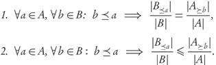
Definition 2.4. For two archives A, B ⊂ X we say that A is well-dominated by B if
1. A is dominated by B, written B ≤ A, i.e., ∀a ∈ A, ∃b ∈ B s.t. b ≤ a,
and
2. B contains only dominating points, i.e., ∀b ∈ B, ∃a ∈ A s.t. b ≤ a.
If, in addition,
3. ∃b ∈ B\A, ∃a ∈ A\B such that b a,
we will say that A is strictly well-dominated by B.
The Averaged Hausdorff Distance Let (X , d) denote a general metric space X carrying a distance function, or metric, d : X x X → ℝ +, satisfying the standard properties of non-negativity with identity of indiscernibles, symmetry, and the triangle inequality.
Definition 2.5. For x ∈ X and arbitrary A, B ⊂ X, the Hausdorff distance dH(•, •) is defined by extending d to subsets of X through the following steps:
A distance between points and sets: d(x,A):=inf {d (x,a) |a ∈ A}.
A pre-distance between sets: d(B,A):=sup {d (b,A) | b ∈ B}.
The Hausdorff distance between sets: dH(A, B) := max {d(A, B), d(B, A)}.
It is well-known that endowed with dH, the set K(X) ⊂ -P(X) of all non-empty compact subsets of X turns into a metric space itself. Moreover, (K(M), dH) is a complete metric space if (X, d) is also complete (cf. [4]).
In our context, the metric space under consideration will always be a subset X ⊂ ℝ n (or ℝ k) endowed with the Euclidean distance d(x, xz) := ||x - x'|| induced by its standard 2-norm.
Definition 2.6. For p ∈ N, and finite subsets A, B ⊂ ℝn the (modified) Generational Distance between them is given by
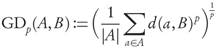 ,
,while the (modified) Inverted Generational Distance is
Finally, their Averaged Hausdorff Distance is defined as

The indicator Δ p can be viewed as a composition of slight variations of the Generational Distance (GD, see [13]) and the Inverted Generational Distance (IGD, see [2]). From X p the standard Hausdorff distance can be obtained as limp→∞ Δ p = d H , but for finite values of p the indicator Δ p returns a p -power mean or p-average of the distances considered for dH.
Performance Indicators Let Y = F (X) ⊂ ℝk be the objective space of a MOP. In this context, a performance indicator is a function J: P (Y) → ℝ+ used to measure the suitability of solution sets. In standard terminology, such an indicator is said to be Pareto-compliant if for subsets F (A), F (B) ⊂ Y the strict dominance condition A ≤ B and B  A implies the inequality J(F(A)) ≤ J(F(B)), or a stronger sense when it implies I(F(A)) < J(F(B)). Additional details can be found, e.g., in [15] (see also [3] and [14]).
If A ⊂ X denotes a candidate archive, the explicit values of the GDp, IGDp, and Δ p -performance indicators assigned to A are given, respectively, by
Remark. We will calculate the GDp and IGDp distances between subsets of the objective space Y = F(X) that are images through F of subsets A ⊂ X which, by definition, are assumed to consist of mutually non-dominated points (like archives or the Pareto set itself). This implies that the restriction F|A: A F(A) is injective, thus a bijection onto its image. Since |A| = |F(A)|, in the finite case the elements of F(A) can be labelled by those of its preimage A in decision space X ⊂ ℝn, and all sums will appear over subsets of X.
In practice, additional assumptions on the sets of comparable archives may be necessary for the required inequalities of Pareto-compliance to hold, and even knowledge on the behavior of the underlying Pareto set P, or its front F(P), can be necessary. Although, in real applications, information on the Pareto set is not usually obtainable, from a purely theoretic point of view those assumptions can help to determine the usefulness of an indicator by elucidating its behavior, and by comparison with known examples.
Compliance to Pareto Optimality
For the Generational Distance We begin by recalling a useful property of GDp -distances proved in [9], and valid for pointwise solutions under simple hypotheses on the Pareto front. Variations of this property will appear as assumptions in the statement of further results on GDp -values for arbitrary finite sets. For calculating the GDp -indicator it is not necessary to assume that P is finite, it can be infinite, continuous, or even piecewise continuous. If necessary, it will be assumed to be compact where explicitly stated.
Lemma 3.1. Let a, b ∈ X ⊂ ℝn and suppose that the Pareto front F (P) ⊂ ℝk is connected, or that for each i = 1,..., k there is an element y (l) ∈ F (P) such that the components y j (i) = f j (b), for all j ≠ i. Then:

Proof. The proofs are direct consequences of [9, Prop. 1, Prop. 2].
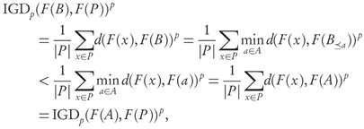
Briefly speaking, the property established by Lemma 3.1 says that if an archive B can be obtained from another archive A by only replacing one dominated solution a ∈ A with a dominating one b ∈ B, the value of the GDp indicator decreases. Namely, if for archives B :={b,x2,...,xn} and A :={a,x2,...xn}, we have b ≤ a, then GDp(F(A), F(P)) < GDp(F(B), F(P)), i.e., the Pareto compliance holds when comparing individual solutions.
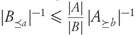
In [9, Prop. 3] the Pareto compliance of the Generational Distance GDp is also considered. In particular, it is stated that for finite archives A, B ⊂ ℝn, where A is well-dominated by B, the extra assumption
 ,
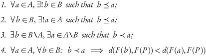
,suffices to ensure that GDp (F(B), F(P)) < GDp (F(A), F(P)). Unfortunately, the last step of the proof is not correct under the generality of the original assumptions. In fact, scenarios shown in Example 3.2 and Figure 1 indicate that the conclusion does not always hold. This is because the behavior of the p-average distance for a dominating archive B, could be worst than the corresponding p-average for a dominated set A having more points in its image close to F(P) than those of B. A remedy to those situations is introduced in Theorem 3.4 by imposing assumptions on the sizes of some dominated/dominating sets of points.
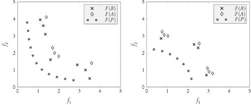
Figure 1 Two different situations where the GD p value of archive A turns out to be better (smaller) than the GDp value of archive B, even though B < A and the original assumptions of Prop. 3 of [9] are satisfied. Notice the number and distribution of dominated/dominating points in relation to F (P).
Example 3.2. A simple case violating [9, Prop. 3]:
Pareto Front F(P):= segment from (0,5) to (5, 0),
Dominated Archive F (A) := {(1, 6), (2, 5), (6, 4)},
Dominating Archive F (B) := {(1, 5), (5, 4), (6, 3)},
Smaller Indicator GD2(F(A),F(P)) = √19.3,
Larger Indicator GD2(F(B),F(P)) = √22.
Nevertheless, a slight modification (regarding the uniqueness of the elements whose existence is ensured by the hypotheses) already makes the conclusion of the original proposition true. The complete corrected statement is a consequence of the more general result stated in Theorem 3.4 and reads as follows
Proposition 3.3. Let A, B ⊂ Rn be finite archives such that:
Then, GDp(F(B),F(P)) < GDp(F(A),F(P)).
Proof. It is a simple consequence of Theorem 3.4 below.
Figure 2 illustrates two examples where the conditions of Proposition 3.3 hold, and therefore, the Pareto-compliance conclusion applies. In both cases, each element of B dominates only one element of A, and each element of A is dominated by only one of B, so that the archives are equal sized. In these examples the assumptions of the original statement in [9, Prop. 3] hold.
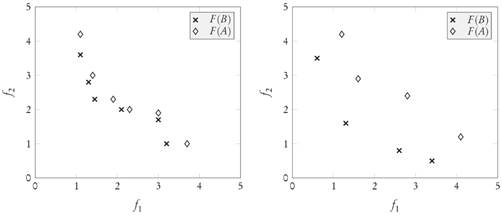
Figure 2 Two different situations where B ≤ A and the adjusted assumptions of Proposition 3.3 arevalid.Inthesecasesthe GDp valueofarchive B is better (smaller) than the GDp value of archive A.
Notice that the only difference between Proposition 3.3 and [9, Prop. 3] is that conditions 1 and 2 ask for the existence of unique dominating (b ∈ B) and dominated (a ∈ A) elements, respectively. Without these clarifications the conclusion can easily become false, but with them there is still the problem that the assumptions turn out to be unnecessarily restrictive. In fact, they imply that the archives A and B have the same size. However, simple cases already presented in [9] and shown in Figure 3 suggest that it should be possible to keep the conclusion under milder conditions.
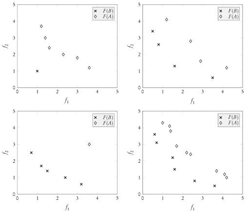
Figure 3 Four different scenarios where the GDp value of archive B is better (smaller) than the GDp value of archive A independently of the Pareto front F(P), and where the additional assumptions made in Theorem 3.4 are easily verifiable.
Our next result provides a general statement from which Proposition 3.3 follows as the simplest non-trivial case.
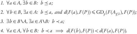
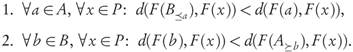
Theorem 3.4. Let A, B ⊂ ℝ n be finite and strictly well-dominated archives with B ≤ A, such that
Then, GDp(F (B),F(P)) < GDp(F(A),F(P)).
Proof. By condition 1, for arbitrary a ∈ A and b ∈ B≤a we have the inequality d(F(b),F(P))p d(F(a),F(P))p. After taking the average over all b ∈ B <a at the left-hand side, we obtain
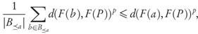
and averaging both sides again over all a ∈ A yields
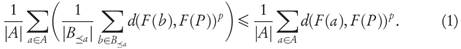
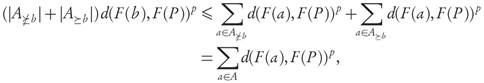
From property 2 we can write the left-hand side as
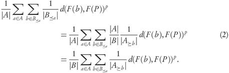
Now, realizing that each b ∈ B will appear |A≥b|-times in the total it becomes
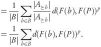
Returning to (1) we conclude that GDp(F(B), F(P))p ≤ GDp(F(A), F(P))p.
Finally, property 3 of Definition 2.4 for strictly well-dominated sets ensures that the inequality has to be strict, and the claim follows.
From the step leading to (2) in the proof of Theorem 3.4 it is apparent that the conclusion is still valid if we change the “=” sign between the involved ratios |A| in condition 2 by “≤”, because then
 , and (2) becomes a “≤’’-inequality. Nevertheless, the following result asserts that there is no difference in making that change.
Lemma 3.5. Let A, B ⊂ ℝn be finite archives. Then, assuming all the involved sets are non-empty, the following conditions are equivalent:
Proof. Clearly 1 implies 2. For the converse, using 2 with any b ≤ a we have the inequality

It is clear that if at both sides of (3) we take the sum over all a ∈ A and b ∈ B for which b ≤ a we find that,
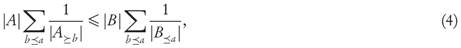
where the left-hand side of (4) can be rewritten as
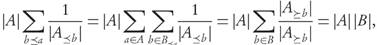
and similarly for the right-hand side we have
Hence, both sides of (4) are actually equal. This could not have been the case if for some b ≤ a the inequality (3) were strict, i.e., it has to be always an equality. This implies condition 1.
We end our consideration of the GD p indicator with an alternative form in which the original statement in [9, Prop. 3] can be fixed without asking for unique dominated/dominating elements. The drawback is that it requires previous knowledge on the behavior of the indicator for non-dominating subsets of the dominated archive A.
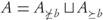
Proposition 3.6. Let A, B ⊂ R n be finite archives such that:
Then, GDp(F(B),F(P)) < GDp(F(A),F(P)).
Proof. Forany b ∈ B, it follows from condition 4 by taking p-averagesoverall elements a ∈ A ≥b that the inequality d(F(b),F(P)) p < GDp(F(A >b ),F(P)) p holds. Moreover, for any a ∈ A ≥b we know using conditions 2 and 4 that
d(F(b),F(P)) p ≤ d(F(a),F(P)) p ≤ GDp (F(A ≥b )),F(P)) p .
Since
 , adding the previous inequalities shows that for any b ∈ B,
in other words, d(F(b), F(P))p ≤ GDp(F(A), F(P))p. Finally, averaging over all b ∈ B yields the conclusion, taking into account that condition 3 ensures the strict inequality.
For the Inverted Generational Distance Now we will concentrate on the Inverted Generational indicator IGDp. In this context we will always assume that the Pareto front F(P) is either finite or a finite size approximation has been chosen to be able to use the expression given in Definition 2.6. The following is a simple property that will be required among the hypotheses of the remaining results.
Lemma 3.7. Let A, B ⊂ ℝn be finite archives and P a Pareto set approximation.

Proof. Suppose that for a ∈ A, b ∈ B, and x ∈ P, we have x ≤ b ≤ a, then d(F(b),F(x)) = ||F(b) - F(x)|| < ||F(a) - F(x)|| = d(F(a),F(x)). This property clearly holds for all x ∈ P ≤b .
Strenghtening the previous property to the whole Pareto set, we obtain our first Pareto compliance criterion.
Proposition 3.8. Let A, B ⊂ Rn be finite and strictly well-dominated archives with B ≤ A and P a finite Pareto set approximation such that

Then: IGDp(F(B),F(P))< IGDp(F(A),F(P)).
In the particular case when an approximation P to the Pareto set satisfies P ≤ B (i.e., P≤B = P) it is clear that the conditions of Proposition 3.8 hold immediately by Lemma 3.7, thus in this case the validity of the Pareto compliance for the IGDp-indicator is guaranteed.
Proof of Proposition 3.8. By the hypothesis, taking succesive infima over all x, x' ∈ P at both sides of the initial inequality, it follows that if F(P) is a compact subset, for all a ∈ A and b ∈ B the dominance relation b < a implies

or only that d(F(b),F(P)) ≤ d(F(a),F(P)) if F(P) were not known to be compact, because in the first case the infimum (actually minimum) at the right-hand side of (5) is reached at some point F(x 0) on the Pareto front F(P), ensuring an strict inequality
d(F(b),F(P)) ≤ d(F(b),F(X0)) ≤ d(F(a),F(%) = d(F(a),F(P)).
Without the compactness assumption, the infimum at the right-hand side could reach the one to its left, but of course this is not the case here with F (P) finite. Finally, using that
 the claim follows from
as stated.
Remark. Notice that in Proposition 3.8 the Pareto compliance of the Inverted Generational Distance IGD p does not depend explicitly on the size of the sets A, B, or their subsets, in contrast to what was found in Theorem 3.4 for the Generational Distance GD p . This is in part due to the strength of the assumption used for this proposition, which in many cases of interest will unfortunately not hold for all x ∈ P. It is clear from the proof that this assumption can be replaced by any of the following slightly weaker ones:
Indeed, the proof using condition 1 is basically the same, and the one using condition 2 just requires to write
 in order to see that

Still, these conditions are strong and do not necessarily apply when B does not cover the whole spectrum of admissible optimal solutions, thus alternatives are desirable.
Figure 4 displays two cases where the assumptions of Proposition 3.8 are valid. In fact, for both of them it is easy to see that P ≤ B ≤ A, so that their validity is a consequence of Lemma 3.7. Whenever these dominance relations hold, the size or form of the archives under comparison do not matter, and the Pareto compliance of the IGD p -indicator is satisfied.
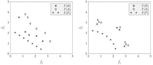
Figure 4 Two different scenarios where the IGDp value of archive B is better (smaller) than the IGDp value of archive A, where the hypotheses of Proposition 3.8 hold.
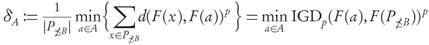
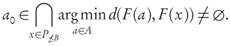
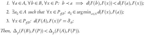
For the following statement, we recall that given a finite archive A ⊂ X and a fixed point x ∈ P there always exists at least one element a0(x) ∈ A such that a0(x) ∈ arg mii a∈A d(F(x),F(a)). The minimal p-average distance between points F(a) and F(P≥B) will be abbreviated by
Theorem 3.9. Let A, B ⊂ ℝn be finite and strictly well-dominated archives with B ≤ A, such that any of the following conditions hold true:
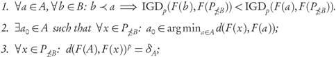
then, IGD p (F(B),F(P))< IGD p (F(A),F(P)).
Proof. First, notice that Lemma 3.7 and Proposition 3.8 imply that we always have IGDp (F(B),F(P ≤B )) ≤ IGDp (F(A),F(P ≤B)). From condition 1, and by a similar calculation to the one in the proof of Proposition 3.8 (but restricted to P ≤B ) it follows that IGDp(F(B), F(P ≤B )) < IGDp(F(A), F(P ≤B )). Since P = P ≤B U P ≤B , the conclusion easily follows in this case by adding |P ≤B | times the first inequality with |P≤B| times the second, and dividing both sides by |P|.
Second, notice that for A ⊂ X the following inequality always holds

because at the left-hand side the minimum of each term may be reached for different a ∈ A, while at the right-hand side the same a ∈ A is required in all terms. For both sides to be equal it is enough (although not necessary) the existence of some fixed a0 ∈ A at which the distance from F ( x ) to F (A) is reached for all x ∈ P ≤B . Explicitly, ∀x ∈ P ≤B : d(F(x), F(A)) = d(F(x), F(a0)). Indeed, in this case both sides of (6) attain the same minimum possible value at the point a0. Before we proceed with the final calculation, notice that from both conditions 2 and 3 we have
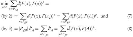
From these observations, and using that P ≤B ≤ B with Proposition 3.8, it follows that
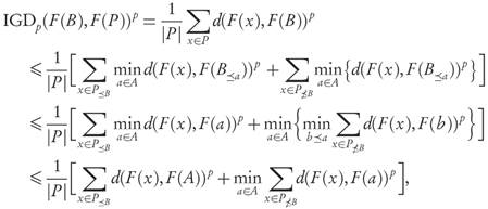
where we used condition 1 to recast the second term. Using (7) or (8) we conclude that
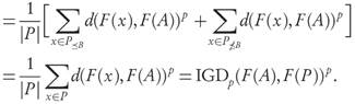
Remark. Condition 2 of Theorem 3.9 requires that for some a0 ∈ A we have
In dimension n = 2, from the fact that A and P consist only of mutually non-dominating points, it is possible to show that the intersection admits more than one element only when |P ≤B | = 1 and |A| > 1, otherwise, the condition is that the intersection should be precisely a0. For n > 2 the situation is, in general, more complicated. Also, condition 3 of Theorem 3.9 can be rephrased by saying that each x ∈ P ≤B has an associated element ax ∈ A at which its distance to A is reached, and for any of those x this distance has the same value δA (given by the average of all distances d(x, a) to points a ∈ A), i.e.,
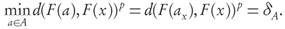
Note that from the definition of as a minimal average, the seemingly weaker condition
 , implies that all the “≥’’-inequalities need to be actual equalities, because a collection of values cannot all be greater than, or equal to their average, unless all are equal to it.
Figure 5 illustrates four situations where Theorem 3.9 applies. At the upper left appears a variant of the second case in Figure 4 where condition 1 holds, while at the upper right the diamond in the corner of F(A) corresponds to the image F(a0) of the point a0 required in condition 2. Finally, both of the lower diagrams correspond to cases where the points of F(P) are equidistant of F(A) so that condition 3 holds, and δA is precisely this distance (to the power p).
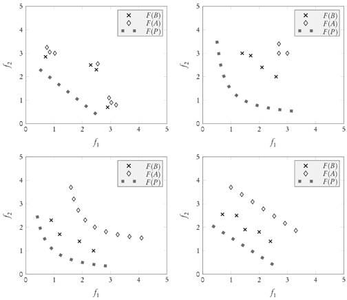
Figure 5 Four situations where the IGDp value of archive B is smaller (better) than the IGDp value of archive A, and where the conditions of Theorem 3.9 are satisfied.
Remark. We conclude our analysis of the IGDp-indicator highlighting useful cases where each one of the assumptions needed for Theorem 3.9 hold, and which are illustrated in Figure 5.
The first condition holds, in particular, whenever P ≤ B ≤ A.
The second condition is valid when the dominated archive A is much more convex than the Pareto front. For example, this can occur if F(P) is concave, or flat, and A is sufficiently convex (i.e., curved in the opposite direction of F(P)).
The third condition holds whenever the Pareto front F(P) and the dominated archive A have corresponding equidistant points.
Consequences for the Averaged Hausdorff Distance Criteria for the Pareto compliance of Δ p can now be stated as a consequence of the compliance of their intermediate generational indicators GDp and IGDp . Using the same notation for as in the previous part, we can add up the results of the previous sections in the following
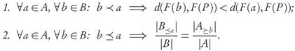
Theorem 3.10. Let A, B ⊂ Rn befinite and well-dominated archives with B ≤ A such that
and any ofthe following conditions hold
Proof. From condition 1 it follows easily that

which is precisely condition 1 of Theorem 3.4, and furthermore, it also implies condition 1 of Theorem 3.9. Hence, this list of conditions satisfy all the requirements of Theorems 3.4 and Theorem 3.9. From the definition of Δ p we immediately arrive at the desired conclusion.
It is possible to study in detail which of the GD p or IGD p -distances to the Pareto front is larger for two candidate archives, in order to find the indicator that will correspond to the value of Δ p in each case. We will not explore this question further, but clearly, if the same indicator realizes the value of Δ p for both archives the compliance can be evaluated through the previously presented results for that indicator alone.
Conclusions and Perspectives
In this study, different criteria have been obtained to establish the Pareto compliance for the averaged Hausdorff distance, anditsassociatedgenerational p-indicators, when dealing with finite solutions/approximations. Inaccuracies found in the current literature have also been corrected, and as far as the constraints and scope of the problem permits, general results have been provided. As an important observation, from Theorem 3.4 and the examples presented, it can be stated that the Pareto compliance of GD p (and therefore of A p ) is not, in general, completely independent on the size ofthe solution sets to be compared (except under very particular circumstances). Additionally, two alternative conditions were given to guarantee the compliance of the IGD p -indicator and that help to elucidate its behavior. Although the conditions depend on the characteristics of the Pareto set under consideration, it is important to note that they are useful in cases where the convexity/concavity of the solutions and/or the expected ones of the Pareto set are known.
As it was already mentioned in the introduction, it is natural to consider generalizations of GD p , IGD p , and Δ p that can enhance their usefulness. Some proposals have already been made for GD p , e.g., in [6], and furthermore, a ( p , q )-averaged Hausdorff distance Δ p,q has been introduced in [12] for the case of finite archives, and in [1 ] for continuous ones, in terms of generalized generational distances GD p,q and IGD p,q suited to each context.
From a theoretical perspective, further consideration of the convenience of those generalizations requiren otonlya deeper understanding of the properties ofGD p , IGD p and Δ p as indicators themselves, butalsoasetofwell-established and testable assumptions allowing for appropriate comparisons. This work is an intermediate contribution to that aim from the purely theoretical side, and its extension to the (p, q)-generalizations is a matter of further investigation.
Apart from EMO algorithms, performance indicators play an important role on all set oriented methods, i.e., methods that generate an entire set of solutions in one run of an algorithm. This is the case, e.g., of subdivision and cell mapping techniques (see [11, 5]). It is a matter of futher study how the results presented here can be extended to those contexts.

