


 text in
  English (pdf)
 Article in xml format
 Article references
 Send this article by e-mail
 Cited by SciELO
  Cited by Google
  Similars in
SciELO
Similars in
SciELO  Similars in Google
 Permalink
INTRODUCTION
The cryosphere is a natural integrator of the variability of the climate and provides some of the most visible records of climate change (Vaughan et al., 2013; IPCC, 2014), based on the variation of solid water such as snow, ice from rivers and lakes, sea ice, glaciers, ice shelves, continental ice, and frozen ground (permafrost). Particularly the Antarctic holds most cryosphere worldwide; therefore, its melting potentially will raise sea level up to 61 m, which would substantially affect a large part of the human population (Moss et al., 2010; Vaughan et al., 2013).
According to the United Nations Framework Convention on Climate Change (UNFCCC), climate change, which has altered the composition of the global atmosphere variating climate observed during comparable periods (IPCC, 2014), is not attributed only by human activity. However, the fifth report of the Intergovernmental Panel on Climate Change (IPCC, AR5) indicated global warming is unequivocally influenced by human activity. During last century average surface temperature has increased from 0.60 to 0.78 °C (Vaughan et al., 2003), and both atmosphere and ocean have warmed up, snow volumes and ice thickness have decreased substantially, and sea level has risen (IPCC, 2013, 2014; IPCCa, 2014).
Although glaciers respond to temperature variation, increasing or decreasing in volume and advancing or retreating in their fronts (Marangunic et al., 2008), almost all glaciers in the world have been continuously reduced since the late 80s, showing negative mass balances as a result of glacier mass loss (e.g. Kejna et al., 1998; Park et al., 1998; Calvet et al., 1999; Simões et al., 1999; Arigony-Neto et al., 2004). Consequently, glaciers have lost mass and have contributed to sea-level rise throughout the twentieth century (Vaughan et al., 2003; Goss, 2020). For example, at West Antarctic the Thwaites glacier in the Amundsen Sea, one of the largest glaciers on the continent, is currently melting because the water below the glacier is currently two degrees above freezing (Goss, 2020), which could raise sea levels by more than half a meter (Rignot et al., 2014), relevant topic to consider due to the relative proximity to the Antarctic Peninsula.
Because of the highest climate change implications related to cryosphere melting, the Antarctic is one of the most studied areas regarding global warming (IPCC, 2013), mainly the Antarctic Peninsula, where has been reported the highest temperatures in the Southern Hemisphere (Braun, 2001; Vauhghan et al., 2003), showing an increase around 3 °C since 1950 (Meredith and King, 2005). As a result, several studies have provided evidence of glaciers retreatment on the Antarctic Peninsula and in the South Shetland Islands (Kejna et al., 1998; Park et al., 1998; Calvet et al., 1999; Simões et al., 1999; Braun, 2001; Braun and Gossmann, 2002; Arigony-Neto et al., 2004).
Particularly on King George Island (KGI), glaciers are small and temperate, showing temperatures near to 0 °C melting point, doing these ice masses very sensitive to temperature changes (Knap et al., 1996). In the KGI, it has been reported significant air temperature increase, higher ablation rates, and glacier retreatment in comparison to other sites on the Antarctic Peninsula (Braun, 2001). Indeed, during the last 45 years, glacier basin runoff has been increasing on KGI, and since 1956, this island has lost approximately 7 % of its original ice cover (Simões et al., 1999). Only on the Southern coast in KGI, most of the glaciers that flow as continental ice has been receding (Simões et al., 1995, 1999). The KGI ice loss was related to an increase in the estimated average atmospheric temperature (Ferron et al., 2004), matching with regional warming in the South Shetland Islands since 1944 and in the northern part of the Antarctic Peninsula since 1960 (Peel et al., 1988; Braun, 2001). Particularly, the front of the Lange Glacier (LG), located on the Southern Coast of the continental ice, has retreated 1 km over 35 years, evidenced by aerial photographic records, topographic maps, and satellite images obtained in 1956, 1988-89, and 1991 (Simões et al., 1995, 1999; Macheret and Moskalevsky, 1999).
With the purpose to obtain data and information on the dynamics and melting in the LG, we used a network of stakes with temperature data loggers and Sentinel-1 satellite images. Furthermore, a CTD (conductivity, temperature, and density) equipment was deployed in the Admiralty Bay, to assess water surface temperature and salinity in the water column in the bay facing the glacier. Additionally, a bathymetric survey was carried out in the glacier front to determine the depth and ice thickness to estimate its flow dynamics and surface melting. All these data together will provide a current diagnosis of the LG in the current scenario of climate change, which influences the temperature increasing of Antarctic Peninsula and is positively related to the loss of ice and melting in this area (Vaughan et al., 2013). This work provides new knowledge related to the Sustainable Development Goal No. 13 about Climate Action of the United Nations Development Program, and it is framed within the research guidelines of the Scientific Committee on Antarctic Research - SCAR.
MATERIALS AND METHODS
The fieldwork of this study was carried out within the framework of the research projects of the Fifth Scientific Expedition of Colombia to the Antarctic “Admiral Campos” austral summer 2018 - 2019, the 55th Chilean Antarctic Scientific Expedition (ECA 55) austral summer 2018 - 2019, and 26th Peruvian Antarctic Scientific Expedition austral summer 2018 - 2019.
Study area
King George Island (KGI) is located at the northern portion of the Antarctic Peninsula in the South Shetland Islands Archipelago, between 61° 54’ - 62° 16’ S and 57° 35’ - 59° 02’ W (Ferron et al., 2004) (Figure 1). Eight permanent research stations, various seasonal huts, and research camps are located on KGI, and about 90 % of the island’s surface (1,250 km2) is glaciated (Rückamp et al., 2011). The island’s ice cover consists of several connected ice caps with pronounced outlet glaciers. While the northern coast exhibits gentle slopes, the southern coastline has steeper slopes and fjord-like inlets (Rückamp et al., 2011). The LG is located in the southern portion of KGI, in the Admiralty Bay, in parallel and near the Antarctic Peninsula (Figure 1).
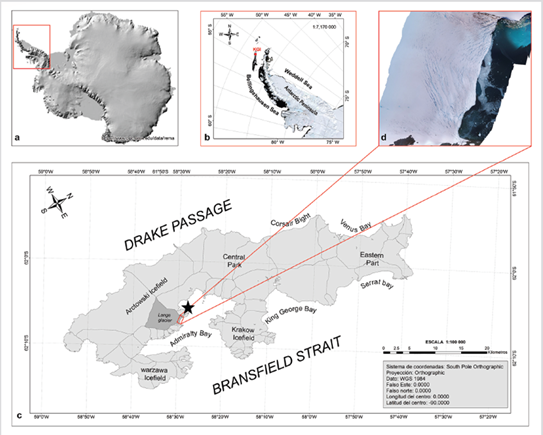
Figure 1 a. Location of the Antarctic Peninsula in the Antarctic continent (map source: Howat et al., 2019 www.pgc.umn.edu/data/rema). b. The map shows a detail of the Antarctic Peninsula, and c. location of the Lange Glacier (LG), in the King George Island. On this last map is marked with a black star the Scientific Antarctica station Machu Picchu of Peru - ECAMP, which is located close to the LG and where the tidegauge was located. The map b. shows an Orthophoto of LG.
The LG is identified as one of the main outlets of ice on KGI, which flows into Admiralty Bay (Barboza et al., 2004) (Figure 1c). This glacier is 6.2 km along the longitudinal axis, 5 km wide in the middle part, its front has a width of approximately 2 km, and its drainage basin covers 28.3 km2 (Barboza et al., 2004). The surface water in front of this glacier is cold and fresh due to the seasonal ice-melting, showing temperature and salinity ranges between -0.13 to 0.79 °C and 32.43 to 33.73, respectively. The measurements in the field and the presence of sediment plumes in the glacier front indicates it is a temperate glacier (Macheret and Moskalevsky, 1999; Pichlmaier et al., 2004), whose basal bed is near to fusion point allowing its glide and basal melting (Marangunic et al., 2008). The LG has high retreatment on its front since 1956 (Simões et al., 1999; Braun, 2001), with a 1.4 km retreat, losing a total of 2.0 km2 (Arigony-Neto, 2001). In front of the LG is located the Admiralty Bay that has a variable bathymetry, which is shallower near to the glacier front with depths between 10 to 220 m (Figure 5), increasing from 300 to 1,000 m in adjacent sub bays. From the central portion of the bay to the output towards Bransfield Strait, are located deeper points with depths between 1,200 and 1,800 m.
Thermic gradient and glacier dynamics
In order to evaluate the thermal gradient on the surface of the glacier, an Onset HOBO temperature data logger sensor was installed in three bamboo stakes (Figure 2a) at 200 m distance each, and 200 m from the northside on the surface of the glacier, on December 24, 2018. Each stake registered temperature data every 10 min during the study period (22 days). We used a Kovacs drill to open a hole and install one stake (Figure 2b). This methodology was conducted to install all stakes, which were georeferenced using a Global Positioning System (GPS). Each stake was measured from the surface-exposed base until its superior end (Figure 2c), to assess variation in ice thickness posteriorly. On January 14, 2019, we re-measured the stake’s position using a GPS to assess glacier velocity.
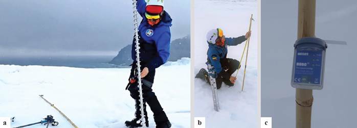
Figure 2 Methodology to install bamboo stakes on the Lange Glacier (LG), KGI, Antarctica. a. Use of Kovacs drill for hole opening and bamboo stake installation. b. Measurements of melt at ablation stake. c. Temperature data logger sensor installed on stake. Photos: a. - b. Jhon Mojica and c. Diego Mojica, 2019.
The dataset from temperature data loggers in each stake was downloaded through the Onset HOBO software version 3.7.13 (https://www.onsetcomp.com/hoboware-free-download). In order to compare and obtain a climatic trend of the area’s temperatures on the LG, we used an Automatic Weather Station (AWS) dataset from the Scientific Antarctica station Machu Picchu of Peru (ECAMP), located close to the LG (Figure 1). Additionally, we used temperature climatological dataset from other AWS (e.g. Ferron et al., 2004; Turner et al., 2005; see Table 2), and the temperature dataset from Frei Station (1970 - 2015) provided by Dr. Jorge Carrasco of the University of Magallanes, Chile (Table 2).
To confirm our results of the methodology used by glacier dynamics, data obtained from the displacement of the three stakes installed was compared with data obtained from Sentinel-1 satellite images. These images were filtered through Copernicus (https://scihub.copernicus.eu/dhus/#/home) of the European Space Agency. For this, we used the level-1 of Ground Range Detected (GRD) products, which consist of focused Synthetic Aperture Radar (SAR). These data were detected, multi-looked, and projected to ground range using an Earth ellipsoid model such as WGS84. The ellipsoid projection of the GRD products was corrected using the terrain height specified in the product general annotation. The terrain height used varies in azimuth but is constant in range (Lu and Veci, 2016).
We work on two satellite images of the study area corresponding to the LG, which were captured at different times during the austral summer (January 19, 2019, and February 24, 2019). The image that was acquired earlier is selected as the “master image” and the other image is selected as the “slave image” (Lu and Veci, 2016). These images were subsequently analyzed using the Offset Tracking SAR in the Application of Sentinels Application Platform (SNAP). Offset Tracking is a technique that measures feature motion between two images using patch intensity cross-correlation optimization and has been widely used in glacier motion estimation (Lu and Veci, 2016).
Calculation of width and frontal area of Lange Glacier
In order to assess the depth and thickness of the LG under the sea and show historical variations (e.g. Arigony-Neto, 2001; Braun, 2001; Barboza et al., 2004), we used a Defender-type boat, provided from Colombian vessel “ARC 20 de Julio” to conduct this bathymetric survey, an activity supported by the Colombian Antarctic Program, the National Navy of Colombia, and the General Maritime Directorate (Colombian Maritime Authority). We used a multibeam echo sounder Kongsberg of 80 and 200 kHz to capture data with greater spatial coverage and frequency. Also, a tide gauge installed in the vicinity of the LG was used (62° 05’ 29” S, 58° 28’ 06” W) (Figure 1c). The acquisition and processing of the dataset were carried out using the CARIS Easy View 4.4.1 and HYPACK software. We also used bathymetric data provided from Peruvian vessel “BAP Carrasco”, from the Navy of Peru and Peruvian Antarctic Program.
In order to estimate the current ice thickness and width of the LG front above sea level, a Digital Elevation Model (DEM) was performed using a Remotely Pilot Aircraft (RPA) technology, which was geodesically adjusted with the static method (2 hours - 1per every 5 seconds), and an orthophoto (georeferenced and scale image of the territory) was generated in ArcMap 10.3. To calculate the glacier frontal area, 10 m inwards of the glacier was taken to generate curves in the Digital Surface Model (DSM), with an interval of 0.5 m of equidistance to produce a Triangular Irregular Net (TIN), and we generated a Polygon Volume in ArcGIS 10.3.
Calculation of Calving flux
We estimated the LG calving flux using previous data from stakes movement, bathymetric survey, and DEM, following this equation:

Where Q C is the Calving flux (Motyka et al., 2003, Benn et al., 2007). S represents the glacier frontal area, which was calculated adding up both emerged and submerged glacier front areas. To assess the emerged area of glacier front we used glacier front width data obtained with DEM and ArcGIS; to estimate the submerged area of glacier front, we averaged depths obtained with a bathymetric survey, and this value was multiplied with the value of glacier front width over sea level. U T corresponds to velocity of the glacier front, which was assessed using both superficial and basal velocities. Superficial velocity was determined from measurements of stake positions at the beginning and the end of the study period and basal slip speed was averaged at 50 % because this type of glaciers (temperate) usually shows velocities between 40 % and 60 % (Marangunic et al., 2008). dx/dt is the change in glacier frontal position (e.g. Sikonia, 1982; Bindschadler and Rasmusen, 1983; Van der Veen, 2002; Vieli et al., 2002; Siegert and Dowdeswell, 2004), which was estimated using historical data of width glacier front reported by Barboza et al. (2004) to compare with current data calculated using the DEM.
Oceanographic stations
We collected all oceanographic data on December 24, 2018, recording all datasets in a short period to characterize the ocean-glacier dynamic as a quasi-steady system. The equipment used was a CastAway CTD (https://www.sontek.com/castaway-ctd) that provides profiles of temperature, conductivity (salinity), and sound speed at different pressure (depth). The temperature accuracy is +0.05 °C, salinity +0.1 PSU, and pressure +0.01 dBar, with a sampling rate of 5Hz determined by the manufacturer. The profiles were recorded in front of the LG, northeast and central part of the bay.
To analyze the oceanographic data, we split the CTD stations into two sections, one parallel and perpendicular regarding the glacier front (Figure 3). The further station was located at 1 km from the glacier front southeast direction. Due to ice-cover, the southern part of the glacier front was not covered by the CTD measurements. A total of 29 usable CTD profiles were included in this study, to characterize the dynamics of the water column. The dataset was processed by the manufacturer software (V1.6) and plotted using the Ocean Data View 4.4. As the dataset was recorded in the summer season, is not representative of the winter dynamics, but allows us to identify trends of the year-round water circulation.
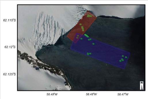
Figure 3 Location of the CastAway-CTD stations recorded in front of the Lange Glacier (LG), King George Island, Antarctica (green dots). The reddish rectangle represents a parallel section (=), and the bluish rectangle indicates a perpendicular section (□) to the glacier front.
In order to describe the ocean dynamic in front to the glacier, we calculated some derived variables, which include: 1) the Brunt Vaisala frequency, to identify the buoyancy of the waters that describes the levels of stability in the system and can help drive the thermohaline circulation in the area (Llanillo et al., 2019); 2) the Turner angle, which defines the levels if the water column conditions are prone to develop unstable processes such as double-diffusion, convection, and salt fingering; and 3) the thermobaric coefficient, which identifies the influence of the water composition and the ratio distribution between the temperature and salinity.
RESULTS
Thermic gradient and glacier dynamics
The glacier dynamics were identified with the displacement of each stake in relation to its initial and final GPS location. The stake one recorded a movement of 10.19 m with direction 155° southeast (SE), the stake two a movement of 9.17 m with direction 110° (SE), and the stake three a movement of 7.11 m with direction 90° (SE) (Figure 4).
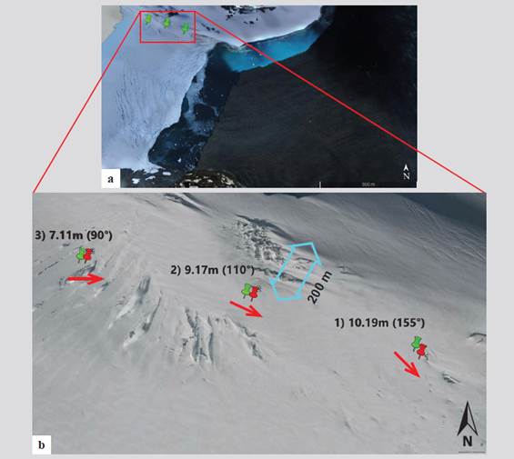
Figure 4 a. - b. Dynamics of the three stakes installed on the Lange Glacier (LG), King George Island, Antarctica. Green markers show the initial position, and red markers show the final position. Blue arrow represents stakes installation distance from the north edge of the glacier. Images: a. DEM and b. Google Earth Pro, 2019.
The network of stakes registered an average movement of 8.8 ± 1.5 m from the initial point of installation (December 24, 2018) to the final measurement point (January 14, 2019) in SE direction towards the front of the glacier, equivalent to 0.40 ± 0.07 m/day, and the Offset Tracking showed a speed of 0.43 ± 0.01 m/day for the stakes installation sector (Figure 4). The detected ice reduction data on stake one, two, and three showed a reduction of 10.5 cm, 8 cm, and 9.5 cm, respectively, showing an average ice thickness loss of 9.3 ± 1.3 cm equivalent to 0.42 ± 0.06 cm/day (Figure 5).
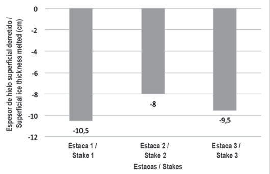
Figure 5 Superficial ice thickness melted from the measurements of the stakes installed in the Lange Glacier (LG), Antarctica, during 22 days from December 24, 2018, to January 14, 2009, in the austral summer 2018 - 2019.
The temperature sensors recorded an average temperature of 5.0 ± 5.2 °C, with minimum temperatures between -2.3 and -2.6, and maximum temperatures between 19.4 and 19.9 °C (Table 1). Conversely, ECAMP registered an average temperature of 1.2 ± 0.7 °C, with a minimum temperature of -1.4 °C and a maximum of 5.6 °C.

Calculation of width and frontal area of Lange Glacier and Calving flux
The bathymetry recorded in the bay in front of the LG showed depths between 10 and 220 m (Figure 6). The deepest zone is located in a small sector in the northeast (NE), at the central part of the glacier front. A shallow zone of 20 m depth is located at 1 km from the glacier front (Figure 6a - b). The orthophoto generated showed that LG front wall length is around 1.4 km (Figure 6c).
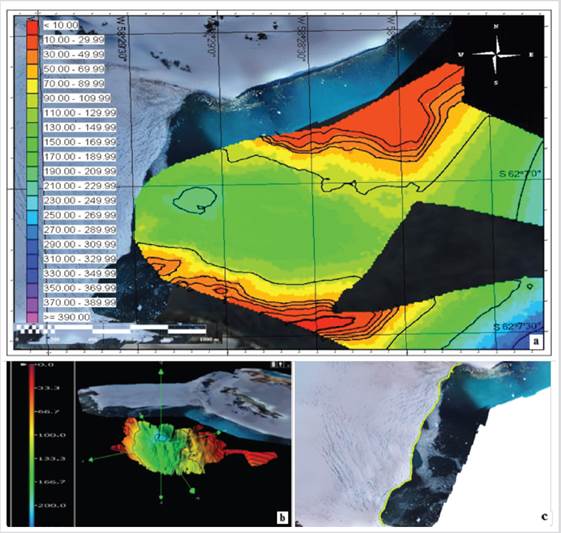
Figure 6 a. Area of the bathymetric survey and Digital Elevation Model (DEM) in front of the Lange Glacier (LG), Admiralty Bay, King George Island, Antarctica. Legend in meters. Blue ellipse in the green central area indicates the deepest point in front of the bay. b. The three-dimensional model of LG; legend is showing in meters (Images obtained from CARIS Easy View, Dirección General Marítima). c. DEM Orthophoto generated by ArcMap 10.3., in which the yellow line represents the glacier front (Instituto Geográfico Nacional del Perú).
The front of the LG was estimated at 198,079 m2, including both submerged and emerged areas. The submerged area of the glacier front was estimated at 137,805 m2, with an average depth of 96.30 ± 53 m and a width of 1,431 m. Regarding the emerged area, it was estimated at 60,274 m2. The estimated velocity of the glacier front was 219 m/yr and its position retreat was 48 m/yr, which showed a Calving flux (Q C ) of 33.87 × 10⁶ m3/yr.
Oceanographic stations
The vertical structure of the LG front is presented on the T-S diagrams (Figure 7). The surface water (~7 m) is cold and fresh due to the seasonal ice-melting, recording minimum values -0.13 °C and 32.43 for temperature and salinity, respectively. Over the 40 m depth was registered the maximum temperature (0.79 °C). Below the seasonal layer, the salinity range is small (33.56 - 33.73) with some variations in the potential density for selected stations.
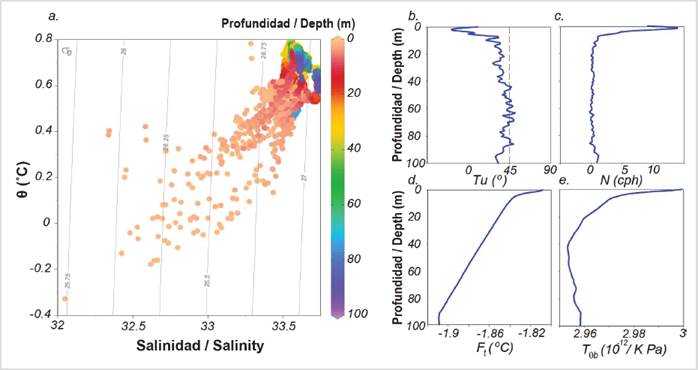
Figure 7 a. T-S diagrams, and an average of the full profiles for b. Turner angle, c. buoyancy frequency, d. freezing temperature, and e. thermobaric coefficient, from all CTD stations in front of the Glacier Lange (LG), Antarctica.
A weakly stratified water column is defined by the lowest buoyancy frequency values, regarding the ocean average (Naverage= 3.0 cph) (Garret and Munk, 1979). This condition was identified below the seasonal surface layer, making the water column prone to lose its stability as it was shown by the Turner angle in specific depths below the 40 m. At this depth, the thermobaric coefficient reached the minimum values of 2.95 x 10⁻¹². This value relates to the highest thermal expansion and the lowest salinity contraction of the water column that decrease the water column stability. The freezing temperature is lower than the water, with no ice depth expectation.
DISCUSSION
This research is the first glaciology study conducted by the Colombian Antarctic Program, with support of Chilean and Peruvian Antarctic Programs, as well as American institutions, to provide recent data about dynamics of Lange Glacier (LG), located in one of the most affected areas by global warming in the Antarctic Peninsula (Vaughan et al., 2013). Our results combined show a high glacier dynamic, associated with a continuous melting by higher temperatures, which could have implications in sea level rise.
Thermic gradient and glacier dynamics
The LG, which has been described as a temperate glacier (Braun, 2001), showed an average superficial movement of 8.8 m ± 1.5 m per 22 days (equivalent to 0.40 ± 0.07 m/day), indicating a displacement of 146 m per year, which is consistent with maximum velocities reported for temperate glaciers (between 10 and until more of 100 m per year; e.g. Lliboutry, 1956). Particularly, glaciers that come from an extensive ice mass and flows into the sea show higher velocities than glaciers inside the Antarctic (Lliboutry, 1956). For instance, the dynamic reported for the Union Glacier in the inside Antarctica showed a slower dynamic between 0.06 and 0.10 m per day, with a mean value of 22.6 m per year (Rivera et al., 2010, 2018). Variations in glacier velocities between exterior and the interior Antarctic could be related to higher temperatures recorded in the Antarctic Peninsula and the South Shetland Islands (Vaughan et al., 2013), differences in dynamic also be related to glacier characteristics, showing higher velocities in the glacier center than the glacier edge (Tarbuck et al., 2005; Marangunic et al., 2008).
Although in our study the stakes were located around the glacier edge (Figure 4b), the dynamic registered was slightly higher than in the center. According to data obtained from offset tracking, satellite images reported a velocity at 0.30 ± 0.03 m/day in the glacier center, while in the glacier edge reported a velocity at 0.43 ± 0.01 m/day (Figure 8), corroborating the results obtained with the installed stakes of 0.40 ± 0.07 m/day. These small differences registered between glacier center and edge may be due to small-scale variations of snow depth induced by crevasse patterns, topographic effects in the area, which vary between center or edge of a glacier (Braun and Hock, 2004), and also due to the change in elevation and more pronounced inclination in the places of installation of the stakes (Wang et al., 2017).
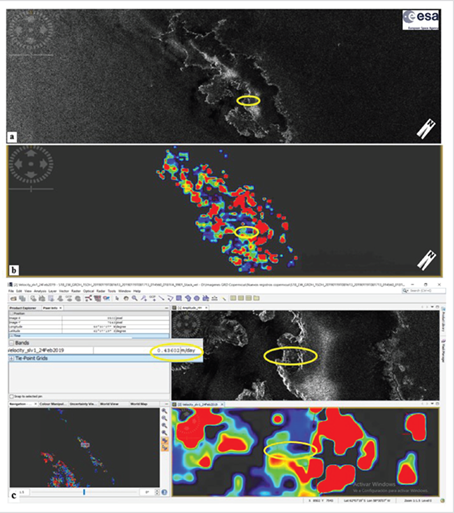
Figure 8 a. King George Island (KGI) satellite “master image”, Antarctica captured on January 19, 2019 by the Sentinel-1 - Mission, and download from Copernicus Open Access Hub by European Space Agency (ESA). b. The image resulting from the Synthetic Aperture Radar (SAR) Application Offset Tracking in Sentinel Application Platform (SNAP). c. SNAP window, for the processing of the acquired satellite images (01192019 “master image” and 24022019 “slave image”) for the LG in KGI. Yellow oval corresponds to the area and velocity m/day recorded in the place where the stakes were installed.
The LG showed an average ice loss of 0.42 cm/day, which is lower than reported by Braun and Hock (2004) in the western part of the ice cap on KGI (average = 0.62 cm/day), who used a total of 15 stakes to monitor ablation in several glaciers including the LG. Although these authors did not install the stakes on LG in the same area of this study, our findings suggest that glacier melting has decreased in recent years. However, melting values reported in this study were higher than reported inside Antarctic (0.04 cm/day in the Union Glacier) (Rivera et al., 2010). The LG is a drainage glacier with an outlet that emerges from a partially drained ice cap (Simões et al., 1999); therefore, and due to global temperature increase tendency, velocity in this glacier may increase in comparison to ice masses inside the Antarctic.
The high temperatures recorded by sensors in the stakes on the LG, which 85 % were above the 0 °C melting point, may increase glacier velocity in the long term. However, this temperature dataset was higher than the data recorded by the AWS of ECAMP during the same season. Comparing the temperature recorded with the stakes with the one obtained from the ECAMP, results showed differences in terms of minimum, maximum, and average temperatures (Table 1). These differences could be attributed to sensor exposition since ECAMP uses a temperature sensor ventilated with a rotor that sucks air to have the most real data of the place, while sensors on stakes can be affected by a local greenhouse effect in the plastic shells that cover them. In other words, sensors on the stakes may be affected by the strong effect of albedo by glacier exposure. Nevertheless, despite these differences between sensor types, both showed most temperatures above 0 °C melting point.
These temperature findings are in concordance with austral summer annual temperature averages reported by stations located in the Antarctic Peninsula such as Bellinghausen, Comandante Ferraz, Esperanza, and Frei between 1944 and 2015 (e.g. Marshall et al., 2002; Ferron et al., 2004; Turner et al., 2005), which are all above 0 °C melting point (see Table 2). In general, historical annual temperature data between 1957 and 1982 from Antarctica shows a warming trend of approximately 1.45 °C (Raper et al., 1984), particularly in the Antarctic Peninsula (Ferron et al., 2004). Indeed, The KGI shows the warmest trend of approximately 2 °C between 1947 and 1997 (50 years) (Smith et al., 1996; King and Harangozo, 1998).
Table 2 Annual and seasonal temperature averages (°C) by decade for Automatic Weather Stations (AWS) located on King George Island and near Antarctic Peninsula.
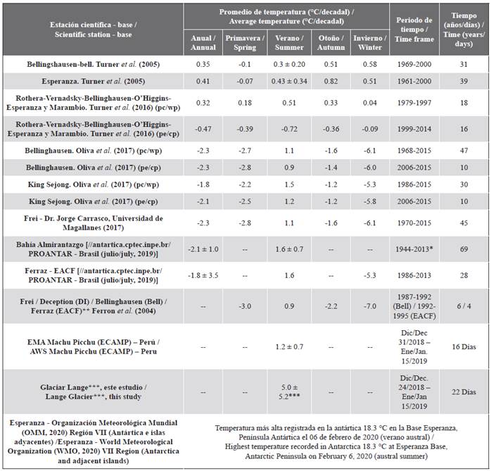
(wp) warm-up period, (cp) cooling period* Except for 1946, data were taken from Deception Island (1944-1945, 1947, 1959-1967), Base “G” (1948-1960), Bellinghausen (1968-1976), Arctowski (1977-1985, 1988-1989), Ferraz (1986-1987, 1990-2013) Source: Data taken from http://antartica.cptec.inpe.br/ Antarctic meteorological PROANTAR - Brazil.** Distance between DI and BELL is 123 km and BELL and EACF are 31.5 km.*** Average temperature for the period described in the table.
However, more recent studies such as those of Carrasco (2013), report a period of slight cooling in the northern part of the Antarctic Peninsula. Oliva et al. (2017), report for the KGI in austral summer an annual mean in air temperature (December to February) lower by 0.3 °C in the decade 2006 - 2015 than in the period 1986 - 2015, in the same way Turner et al. (2016) reported for the Antarctic Peninsula after the warming period between 1979 - 1997, a cooling period, between 1999 - 2014 consistent with natural variability. However, recently the World Meteorological Organization (2020), reported on February 6, 2020, the highest temperature recorded in Antarctica: 18.3 °C at the Esperanza Base (northern part of the Antarctic Peninsula - vicinity of the KGI) (Table 2). All these historical values of temperature in the area together with the results of the measurements of this study indicate a trend of temperature increase with a slight cooling period for approximately 10 to 15 years, according to the latest records could resume the trend of increase of temperature in the Northern portion of the Antarctic Peninsula. This warmer trend in temperatures has direct implications on the current melting of the LG, may continue to retreat if current temperature increase trends increment, contributing to the fresh water inlet to the Admiralty Bay with incidences in the increase of the sea level and all its repercussions in the Coastal zones of the planet.
Oceanographic stations
The surface water was cold and fresh, by Calving and melting processes. At the southern stations, we identified a high salinity and low temperature as a product of the brine produced by the ice formation, in agreement with the visual observations and the lack of data in this area because of the ice-cover (Figure 9). From the parallel section, there was a remarkable area of high temperature (0.78 °C) between 20 and 60 m in the bay central part, associated with low salinity (33.52). Comparing with the perpendicular section (temperature and density signature, Figure 9e-f), we can interpret that this core of warm and freshwater coming from waters outside the Glacier Bay. Comparing the incoming water with the resident, there is a peak of 0.3 °C of variability that can impact directly the glacier front. This statement is relevant for the stability conditions of the glacier because the entrance of this core of waters can produce a subsurface melting process increasing the glacier retreatment, as was presented in previous sections.
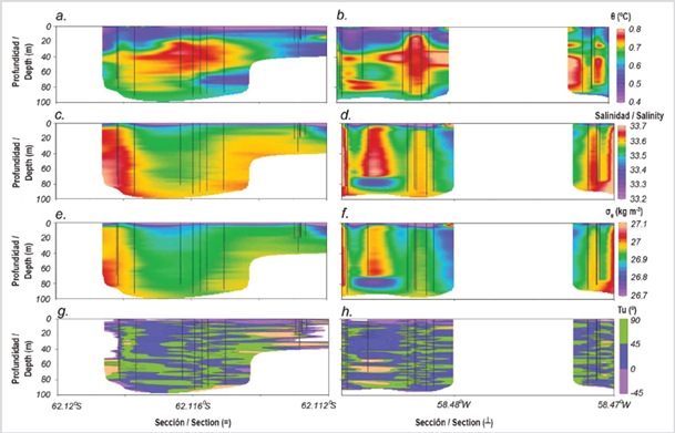
Figure 9 a. - b. Sections of potential temperature, c. - d. salinity, e. - f. potential density, and g. - h. Turner angle for the stations in Admiralty Bay, Antarctica inside each parallel and perpendicular section, respectively.
Cold waters over warm waters, in a weak stratified system, is known as part of the preconditions of convection processes. Consequently, the ocean circulation transport oceanic heat through a weakly stratified water column increasing the surface ventilation (Schmitt, 1994). From this assumption and the Turner angle values and hotspots identified over the water column (Figure 9), we can confirm the entrance of external water making a loss the stability of the water column system. The process as salt fingering can increase the convection mixing in the area, affecting the energy exchange that impacts the ocean-glacier processes, but further studies are need it to confirm the dynamics.
The Antarctic Circumpolar Current is an ocean current that flows from west to east around Antarctica, playing an important role transporting and distributing heat and salt, which have effects on the dynamics of ocean ice, affecting the rates of basal melting and retreat of glaciers (Nitsche et al., 2007; Depoorter et al., 2013). The amount of melting produced by the ocean depends on ocean water temperature, which is controlled by the combination of the surrounding ocean thermal structure and the local circulation of the ocean that is determined by winds and bathymetry. As the climate warms and the atmospheric circulation changes, there will be subsequent changes in the circulation and temperature of the ocean, particularly in the circulation of a warmer layer of water (Circumpolar Deep Water - CDW), which is denser due to the higher salt content and found at depths below surface waters, around 500 m (Holland et al., 2020). This CDW is affecting the glaciers’ frontal retreat, particularly in the western Antarctic Peninsula (Jacobs et al., 2012; Depoorter et al., 2013; Cook et al., 2016). Therefore, the warm, salty, and low-oxygenated CDW that mixes with the recently ventilated and modified High Salinity Shelf Water, which is relatively cold, fresh, and is formed in the Weddel Sea to be advected southward along the deep basins of the Bransfield Strait (Torres et al., 2020), maybe intruding the fresh and warmer waters to the Admiralty Bay.
Bathymetry and Digital Elevation Model (DEM)
The bathymetric survey in the bay facing the LG showed a valley shape, in the center of which are the deepest points with 220 m and the thickest ice (Figure 6a-b). We found an area of sediment plumes in the bay in the front of the glacier, which indicate that glacier front is in contact with the basal bed, in agreement with previous studies in the area (e.g. Barboza et al., 2004; Pichlmaier et al., 2004). Likewise, it was observed 1 km from the front of the glacier some shallow areas of 20 m depth in the southwest (SW) and northeast (NE) of the bay (Figure 6a-b), which may correspond to moraines by the glacial rock drag, sediments, and detritus deposited in the bay. These findings suggest that the front glacier has retreated from the past location. Indeed, the current LG front length showed a notable 600 m retreat in comparison to observations of Barboza et al. (2004) on LG front length 20 years ago.
According to historical descriptions of LG retreatment, the first phase of retreat (440 m) was recorded for the period between 1956 and 1975, and the second retreatment phase was recorded in a short period between 1975 and 1979, retreating about 880 m of ice cliff and losing approximately 1.1 km² (Braun, 2001). This process continued posteriorly between 1979 and 1988, when the glacier retreated an additional 280 m, losing another 0.56 km². Between 1988 and 1995, the glacier retreated 180 m, with an area loss of 0.13 km². In total, the glacier retreated about 1,780 m from 1956 to 1995, thus losing approximately 1.7 km² (Braun, 2001). Similarly, Arigony-Neto (2001) recorded a glacier retreatment of 1.4 km², losing a total of 2.0 km2. Based on these historical data, we estimated a retreatment average of 28 m/year for the period in which there was no data of retreatment records between 1995 and 1999, with glacier retreatment estimated at 112 m. Thus, with all these estimations and including data of this study, the LG retreatment estimated between 1956 and 2019 was approximately 2,492 m.
Climate change considerations
Our results suggest a negative mass balance according to the Calving flux, the temperature registered in this study, and the temperature increase in the area in the last decades. The historical data in the area indicate the LG is increasing continuous fusion (0.42 ± 0.06 cm/day) due to the increase in atmospheric temperature with a freshwater contribution to the Admiralty Bay. From the oceanographic station’s data, there are indications of water external intrusion to the bay in front of the LG. Furthermore, there is a core of external warm water, which destabilizes the water column and generates convection processes. That external water entrance can produce higher levels of mixing and energy, transferred from the ocean to the glacier, driving its retreatment and basal melting below the sea surface. Combining the information of the glacier dynamics from satellite image data, bathymetry, topography that showed the already detectable glacier retreatment and indications for a negative mass balance, the LG is a very good indicator of accelerated climatic change effect in the Antarctic Peninsula. A complete study of the entire glacier basin and continuous monitoring is required to establish the water contribution to sea-level rise due to melting of LG, which may be accelerated by climate change if increase current temperature trends.

