


Serviços Personalizados
Journal
Artigo
 Inglês (pdf)
 Artigo em XML
 Referências do artigo
 Enviar este artigo por email
Indicadores
-
 Citado por SciELO
 -
 Acessos
Links relacionados
-
 Citado por Google
 -
 Similares em
SciELO
Similares em
SciELO -
 Similares em Google
Compartilhar

 Permalink
Ingeniería y Universidad
versão impressa ISSN 0123-2126
Ing. Univ. v.16 n.1 Bogotá jan./jun. 2012
A Review of DAN2 (Dynamic Architecture for Artificial Neural Networks) Model in Time Series Forecasting1
Revisión del modelo DAN2 (Arquitectura dinámica para redes neuronales artificiales) en predicción de series de tiempo2
Uma revisão da DAN2 (arquitetura dinâmica para redes neurais artificiais) modo de previsão de séries temporais3
Juan David Velásquez-Henao4
Carlos Jaime Franco-Cardona5
Yris Olaya-Morales6
1This article is the result of the research project Comparison of Computational Intelligence Techniques for Time Series Prediction, Hermes code: 9761. Developed by the research group Grupo de Computación Aplicada, Universidad Nacional de Colombia, Medellín, Colombia.
2Fecha de recepción: 9 de junio de 2011. Fecha de aceptación: 15 de diciembre de 2011. Este artículo se deriva de un proyecto de investigación denominado Comparación entre técnicas de inteligencia computacional para la predicción de series de tiempo, código hermes: 9761. Desarrollado por el grupo de investigación Grupo de Computación Aplicada de la Universidad Nacional de Colombia, Medellín, Colombia.
3Data de recepção: 9 de junho de 2011. Data de aceitação: 15 de dezembro de 2011. Este artigo deriva de um projeto de pesquisa denominado Comparação entre técnicas de inteligência computacional para a previsão de séries de tempo, código Hermes: 9761. Desenvolvido pelo grupo de pesquisa Grupo de Computação Aplicada da Universidade Nacional da Colômbia, Medellín, Colômbia.
4Ingeniero civil, Universidad Nacional de Colombia, sede Medellín, Colombia. Magíster en Ingeniería de Sistemas, Universidad Nacional de Colombia, sede Medellín. Doctor en Ingeniería, Área de Sistemas Energéticos, Universidad Nacional de Colombia, sede Medellín. Profesor asociado, Escuela de Sistemas, Facultad de Minas, Universidad Nacional de Colombia. Director del grupo de investigación Computación Aplicada, Facultad de Minas, Universidad Nacional de Colombia, Medellín, Colombia. E-mail: jdvelasq@bt.unal.edu.co.
5Ingeniero civil, Universidad Nacional de Colombia, sede Medellín, Colombia. Magíster en Aprovechamiento de Recursos Hidráulicos, Universidad Nacional de Colombia, sede Medellín. Doctor en Ingeniería, Área de Sistemas Energéticos, Universidad Nacional de Colombia, sede Medellín. Profesor asociado, Escuela de Sistemas, Facultad de Minas, Universidad Nacional de Colombia. Miembro de los grupos de investigación Sistemas e Informática y Computación Aplicada, Facultad de Minas, Universidad Nacional de Colombia, Medellín, Colombia. E-mail: cjfranco@bt.unal.edu.co.
6Ingeniera de Petróleos, Universidad Nacional de Colombia, sede Medellín, Colombia. Magíster en Ingeniería de Sistemas, Universidad Nacional de Colombia, sede Medellín. Doctora en Economía de los Recursos Minerales, Colorado School of Mines, Colorado, Estados Unidos. Profesora asociada, Escuela de Sistemas, Facultad de Minas, Universidad Nacional de Colombia. Directora del grupo de Mercados Energéticos, miembro de los grupos de investigación Sistemas e Informática y Computación Aplicada, Facultad de Minas, Universidad Nacional de Colombia, Medellín, Colombia. E-mail: yolayam@bt.unal.edu.co.
Submitted on June 9, 2011. Accepted on December 15, 2011.
Abstract
Recently, Ghiassi, Saidane and Zimbra [Int J Forecasting, vol. 21, 2005, pp. 341-362] presented a dynamic-architecture neural network for time s er ie s p re dic t io n which p er fo r ms significantly better than traditional artificial neural networks and the ARIMA methodology. The main objective of this article is to prove that the original DAN2 model can be rewritten as an additive model. We show that our formulation has several advantages: First, it reduces the total number of parameters to estimate; second, it allows estimating all the linear parameters by using ordinary least squares or ridge regression; and, finally, it improves the search for the global minimum of the error function used to estimate the model parameters. To assess the effectiveness of our approach, we estimate two models for one of the time series used as a benchmark when the original DAN2 model was proposed. The results indicate that our approach is able to find models with similar or better accuracy than the original DAN2.
Keywords: Neural networks (computer science), artificial intelligence, logic programming, time-series analysis.
Resumen
Recientemente, Ghiassi, Saidane y Zimbra [Int J Forecasting, vol. 21, 2005, pp. 341-362] presentaron una red neuronal artificial de arquitectura dinámica (DAN2) para la predicción de series de tiempo, la cual se desempeña significativamente mejor que las redes neuronales tradicionales y que la metodología ARIMA. El objetivo principal de este artículo es demostrar que el modelo original DAN2 puede reescribirse como un modelo aditivo. Se muestra que la formulación propuesta tiene varias ventajas: se reduce el número total de parámetros por estimar, permite calcular todos los parámetros lineales usando mínimos cuadrados ordinarios y se mejora la búsqueda del óptimo global de la función de error usada para estimar los parámetros del modelo. A fin de confirmar la efectividad de nuestra aproximación, se estimaron dos modelos para una de las series de tiempo usadas como benchmark cuando el modelo DAN2 original fue propuesto. Los resultados indican que nuestra aproximación es capaz de encontrar modelos con una precisión similar o mejor respecto al modelo DAN2 original.
Palabras clave: Redes neurales (computadores), inteligencia artificial, programación lógica, análisis de series de tiempo.
Resumo
Recentemente, Ghiassi, Saidane e Zimbra [Int J Forecasting, vol. 21, 2005, pp. 341-362] apresentaram uma rede neural artificial de arquite-tura dinâmica (DAN2) para a previsão de séries temporais, que se desempenha significativamente melhor que as redes neurais tradicionais e que a metodologia ARIMA. O objetivo principal deste artigo é demonstrar que o modelo original DAN2 pode ser reescrito como um modelo aditivo. Mostra-se que a formulação proposta tem várias vantagens: se reduz o número total de parâmetros por estimar, permite estimar todos os parâmetros lineares usando mínimos quadrados ordinários e melhora-se a busca do ótimo global da função de erro usada para estimar os parâmetros do modelo. A fim de confirmar a efetividade de nossa aproximação, estimaram-se dois modelos para uma das séries temporais usadas como benchmark quando o modelo DAN2 original foi proposto. Os resultados indicam que nossa aproximação é capaz de encontrar modelos com uma precisão similar ou melhor que o modelo DAN2 original.
Palavras chave: Redes neurais (computadores), inteligência artificial, programação lógica, análise de séries temporais.
Introduction
Nonlinear forecasts can be more accurate than linear models when time series exhibit nonlinearities. Research topics in this area vary from development of new forecast models to comparison of models' performance for different time series, with the objective of determining model accuracy under fixed conditions.
Recently, Ghiassi and Saidane (2005) have developed a new type of artificial neural network named DAN2. Also, this model is used for forecasting six nonlinear time series that are commonly used as benchmarks, and compare the accuracy of DAN2 with other models (Ghiassi, Saidane and Zimbra, 2005). Collected evidences suggest that DAN2 performs better than the ARIMA approach and traditional artificial neural networks (Ghiassi, Saidane and Zimbra, 2005). In a later study, Ghiassi, Zimbra and Saidane (2006) use DAN2 for medium term electrical load forecasting and compare forecasts obtained using DAN2 with forecasts calculated using an ARIMA and a multilayer perceptron. Ghiassi et al. conclude that DAN2 outperforms the competitive models. Gomes, Maia, Ludermir, Carvalho, and Araujo (2006) propose a new forecasting model based on combining the forecasts obtained using DAN2 and the ARIMA approach; the evidences presented indicate that the new model outperforms the individual forecasts obtained with DAN2 and ARIMA. More recently, Ghiassi, Zimbra, and Saidane (2008) compare the performance of DAN2, traditional artificial neural networks and the ARIMA approach for forecasting the short-, medium-, and long-term urban water demand; this study demonstrates the effectiveness of this new class of neural network.
Wang, Niu, and LI (2010) forecast regional electricity load in Taiwan and conclude that DAN2 performs better than regression models, artificial neural networks and support vector machines. Also, DAN2 has been used to forecast electricity prices; Velasquez and Franco (2010) compare the performance of DAN2 with the ARIMA approach when the prices of electricity contracts in the Colombian energy market are forecasted; they conclude that DAN2 is more accurate than the ARIMA model. Guresen, Kayakutlu, and Daim (2011) forecast the NASDAQ index using several nonlinear models including DAN2. Other experiences with DAN2 indicate that this model may be used to solve nonlinear regression (Ghiassi and Nangoy, 2009) and classification (Ghiassi and Burnley, 2010) problems, too.
We propose a modification of the DAN2 model, aimed at improving the network's estimation procedure. In this paper, we revise the mathematical formulation of DAN2, and we prove that the model can be rewritten as an additive model, reducing the number of parameters to be estimated. In Section 1, we revise the architecture proposed for DAN2 and the training algorithm developed by Ghiassi and Saidane (2005). Then, in Section 2, we review the mathematical formulation of DAN2 and propose a training algorithm that simultaneously estimates all linear parameters of the modified DAN2 model. In Section 3, we compare the performance of our approach to the original DAN2 model fitting both models to one of the original time series benchmarks. Section 4 presents our conclusions.
1. The Original DAN2 Model
1.1. DAN2 Original Architecture
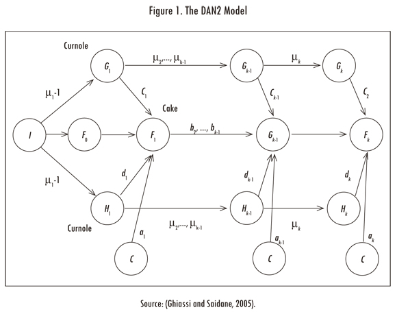
The DAN2 architecture, developed by Ghiassi and Saidane (2005) and Ghiassi, Saidane and Zimbra (2005), is described in this section. The main features of the DAN2 model are depicted in Figure 1. As shown in Figure 1, inputs are presented to the network through the input node I all at once, and not in the sequential process that is the common practice in neural network literature.
There is one linear layer with a unique neurone, F0, which represents a current accumulated knowledge element or CAKE node. Define yt as the time series {y1,...,yt}. The variable X = {Xt; t = P + 1,..., T} is an input matrix where each row, Xt = {xtj; j = 1,...,m} corresponds to the lagged values of the a variable explaining yt. P is the maximum lag considered when we built Xt. The node F0(Xt) is defined as an autoregressive model, such that:

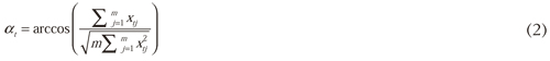
The next hidden layers are composed by four neurones: the first neurone has no input connections and its output always has unit value; this neurone is noted by the letter C in Figure 1. In each hidden nonlinear layer, DAN2 uses a nonlinear transformation based on the projection of over a predefined and fixed reference vector R = {rj; j = 1,..., m } to normalize the data. Here, m is the number of columns of the row vector Xt. For this, the angle, αt, between each data vector Xt and the vector R is calculated. Without loss of generality, R can be defined as a vector of ones as suggested by Ghiassi and Saidane (2005). Thus, the angle αt is calculated as:
Ghiassi and Saidane (2005) prove that this normalization (for the hidden layer k) can be represented by:

Which can be understood as a generalized Fourier series for function approximation. The constant μk is equivalent to a rotation and a translation of the reference vector R and it allows us to extract the nonlinear component in the data. The variation in the value of μk changes the projection of Xt over R and, as a consequence, its contribution to the final solution. Eq. (3) is represented in each hidden layer by two CURNOLE (current residual nonlinear element) nodes. The first CURNOLE node calculates the cosine function (the Gk nodes in Figure 1) and the second node calculates the sine function (the Hk nodes in Figure 1).
The output of each nonlinear hidden layer (and the output layer) is calculated in the CAKE (current accumulated knowledge element) node, Fk, as:

Where αk represents the weight associated to the C node; Ck and dk are the weights associated to the CURNOLE nodes; Fk-1(Xt) is the output of the previous layer, and it is weighted by bk. Eq. (4) defines that the result of each layer is a weighted sum of the knowledge accumulated in the previous layer, Fk-1(Xt), the nonlinear transformation of Xt (Gk and Hk nodes) and a constant (the C node).
1.2. Parameters Estimation for the Original DAN2 Model
The estimation of the model parameters is based on the minimization of an error measure, for example, the sum of squared errors:

The optimization algorithm described by Ghiassi and Saidane (2005) is developed here using the following key points:
- The estimation process is sequential. At first, the parameters of the linear layer defined by Eq. (1) are calculated by ordinary least squares (OLS). While some stop criterion is not satisfied, a new layer is added to the model and fitted to the data. The parameters of previous layers remain fixed.
- DAN2 uses a layer-centered strategy and this means that only the parameters for the new added layer (ak, bk, ck, dk and μk) are optimized with the aim of minimizing Eq. (5).
- In Eq. (4), the sine and cosine functions repeat their values for μk < 0 and for (μk X αt) > 2 πn, such that, it is only necessary to explore values of μk between 0 and max (2π/αt).
- If μk is known, then the other four parameters for the current layer k in Eq. (4) are estimated using OLS; thus, the optimization problem is reduced to estimate the optimal value of μk.
Following the suggestions given by Ghiassi and Saidane (2005), we implement the following strategy for fitting the model to the data:
- Let k = 1.
- For the current layer k, take N points, uk (i), equally spaced over the range of uk, with i = 1,..., N.
- For each point in the grid, !uk (i), simultaneously calculate the parameters 0Ck, bk, ck and dk using OLS and evaluate the fitting error using Eq. (5).
- Keep the value of !uk (i) that minimizes Eq. (5).
- While the error is higher than the minimum admissible error, add new layer to the model; let k = k + 1 and train the new layer following steps 2 to 3.
Note that in step 3 only one set of parameters ak, bk, ck and dk corresponding to the current layer k is estimated and the parameters of the previous layers {aj, bj, cj, dj;j = 1,...,k - 1} remain fixed.
2. The Modified DAN2 Model (mDAN2)
2.1. Proposed Architecture
In this section, we review the DAN2 formulae described by Ghiassi and Saidane (2005) and prove that the model can be written as an additive model, reducing the number of parameters to be estimated, and the required computational resources.
At first, we consider the DAN2 model with only one hidden layer. Thus, we replace Eq. (1) in Eq. (4) with k = 1:
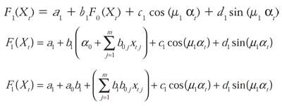
Regrouping terms and substituting a* for a1 + a0b1 and bj* for b1b0j, we obtain:
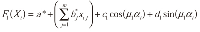
Which describes the output of layer 1 in terms of X. Repeating the described process for layers k = 2,...,K, it is easy to prove that the output for the last layer k is:

In this form, we show that DAN2 can be formulated as an additive model. There are several advantages of using Eq. (6):
The model is lineal for the parameters a*, bl*, ..., bm*, cl*, ..., ck*, dl*, ..., dk* and nonlinear for μk, such that, when the values μ1, ..., μk are known, then the remaining parameters (a*, b*l, ..., bm*, cl*, ..., ck*, dl*, ..., dk*) can be estimated using OLS.
When a new hidden layer is added, we add only three new parameters for the layer instead of the five parameters in Ghiassi and Saidane (2005). As a consequence, the complexity of the estimation of the parameters is reduced. Thus, the final model has 2K less parameters than the original DAN2 model.
2.2. Parameters Estimation for the Modified Architecture
We use a variation of the optimization algorithm described in a previous section:
- Let k = 1.
- For the current layer k, take N points, μk (i), equally spaced over the range of μk, with i = 1, ..., N.
- For each point in the grid, μk (i), calculate the parameters a*, bl* , ..., bm*, cl*, ..., ck*, dl*, ..., dk* using OLS and evaluate the fitting error using Eq. (5).
- Keep the value of μk (i) that minimizes the error in Eq. (5).
- While the error is higher than the minimum admissible error, add new layer to the model; let k = k + 1 and calculate all linear parameters following steps 2 to 4.
Note that the main difference with the original algorithm is the estimation of linear parameters. In the modified algorithm, when a new layer k is added, parameters a*, bl* , ..., bm*, cl*, ..., ck*, dl*, ..., dk* are estimated again along with the parameters for the current layer k, while the μk remain fixed, accumulating knowledge.
3. Numerical Experiment
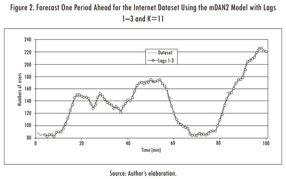
The internet dataset (Ghiassi, Saidane and Zimbra, 2005) was used to test the quality of our approach (see Figure 2). This dataset has a length of 100 observations and it consists in the number of users logged onto an Internet server each minute. The first 80 points are used for fitting the model and the remaining 20 points for forecasting.
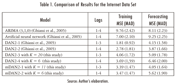
Ghiassi et al (2005) use this dataset for comparing the training and forecasting accuracy of DAN2 against an ARIMA(3,1,0) and a artificial neural network (ANN). For this, two DAN2 models were fitted: the former uses the lags 1_3 as inputs while the second uses the lags 1-4. In Table 1, we reproduce the mean squared error (MSE) and the mean absolute deviate (MAD) reported by Ghiassi et al (2005) for the four models.
We tried to reproduce the errors reported by Ghiassi et al. (2005), but using our own implementation of DAN2. It was impossible to reach equal or lower errors than the reported by Ghiassi et al. (2005) for this time series. We agree with Guresen, Kayakutlu and Daim (2011) when they claim that some parts of the architecture of DAN2 are not clear enough, specially, the fitting algorithms. In a private communication with professor Ghiassi we inquired about the details of the training algorithm; kindly, the professor responded that there is not a free implementation of the algorithm because there is a project for implementing a commercial version of DAN2.
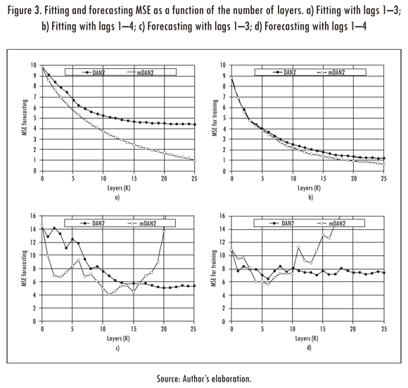
Thus, we trained the original DAN2 model as described in Section 1.2 with a maximum of 25 layers. In figures 3a and 3b, we plot the MSE for the fitting sample as a function of the number of considered layers (K). As is described by Ghiassi and Saidane (2005), the fitting error is reduced each time a new layer is added.
Also, we plot the MSE of DAN2 for the forecasting sample as a function of the number of layers (see Figures 3(c) and 3(d)). The lower forecasting errors are obtained for K = 20 and K = 6 when the lags 1-3 and 1-4 are used as inputs for the model respectively. The errors for the training and forecasting samples are reported in Table 1.
The mDAN2 model was fitted using the same implementation and parameters used for the DAN2 model as described in the previous paragraphs. In figures 3a and 3b. Also, we plot the MSE for the fitting sample as a function of the number of layers. For a low number of layers, the results are similar; but for a big number of layers the difference is high. In all cases (except for k = 0) the mDAN2 model has a lower fitting MSE than the DAN2 original model. Taking into account that we reduce in two the number of parameters of each layer (2K in total), the mDAN2 is preferred in all cases by parsimony. Thus, we prove empirically that our specification is more effective for fitting the data.
Also, we plot the forecasting error for the mDAN2 model (see figures 3c and 3d); a simple inspection reveals that the mDAN2 has a better generalization that the DAN2 original model. Thus, we conclude (for the analysed case) that our representation of the original DAN2 model allow us to find models with a lower fitting error and better generalization; in addition, our model (mDAN2) has a lower number of parameters in comparison with the original version of DAN2. From figures 3c and 3d, we prefer the models with K = 11 and K = 6 layers when the lags 1-3 and 1-4 are used as inputs for our neural network. The MSE and MAD for the fitting and forecasting samples are reported in Table 1. In comparison, the mDAN2 model has a better fitting and generalization that the implemented DAN2 model. Finally, we plot the one step ahead forecast for the mDAN2 with inputs 1-3 and K = 11 in Figure 2.
4. Conclusions
We prove that the "Dynamic Architecture for Artificial Neural Networks" (or DAN2) model can be formulated as an additive model and propose a modification to the original DAN2 estimation algorithm that simultaneously estimates all linear parameters using OLS. The proposed approach has several advantages; first, it decreases the total number of parameters in the model in a factor of 2K; second, all the linear parameters in the model can be estimated directly using OLS; and third, the optimization problem is reduced to obtaining an adequate set of values for . For validating the performance of our approach, we forecast one of the datasets used when the original DAN2 model was validated. We find that our modified DAN2 model performs better than the original DAN2 model using the internet dataset.
References
GHIASSI, M. and BURNLEY, C. Measuring effectiveness of a dynamic artificial neural network algorithm for classification problems. Expert Systems with Applications. 2010, vol. 37, pp. 3118-3128. [ Links ]
GHIASSI, M. and NANGOY S. A dynamic artificial neural network model for forecasting nonlinear processes. Computers & Industrial Engineering. 2009, vol. 57, num. 1, pp. 287-297. [ Links ]
GHIASSI, M. and SAIDANE, H. A dynamic architecture for artificial neural networks. Neurocomputing. 2005, vol. 63, pp. 397-413. [ Links ]
GHIASSI, M.; SAIDANE, H. and ZIMBRA, D. K. A dynamic artificial neural network model for forecasting time series events. International Journal of Forecasting. 2005, vol. 21, num. 2, pp. 341-362. [ Links ]
GHIASSI, M.; ZIMBRA, D.K. and SAIDANE, H. Medium term system load forecasting with dynamic artificial neural network model. Electric Power Systems Research. 2006, vol. 76, pp. 302-316. [ Links ]
GHIASSI, M.; ZIMBRA, D.K. and SAIDANE, H. Urban water demand forecasting with a dynamic artificial neural network model. Journal of Water Resources Planning and Management. 2008, vol. 134, num. 2, pp. 138-146. [ Links ]
GOMES, G. S. S.; MAIA, A. L. S.; LUDERMIR, T. B.; CARVALHO, F. and ARAUJO, A. F. R. Hybrid model with dynamic architecture for forecasting time series. Proceedings of the In-ternationalJoint Conference on Neural Networks. IEEE Computer Society. 2006, pp. 7133-7138. [ Links ]
GURESEN, E.; KAYAKUTLU, G. and DAIM, T.U. Using artificial neural network models in stock market index prediction. Expert Systems with Applications. 2011, vol. 38, pp. 10389-10397. [ Links ]
WANG, J.; NIU, D. and LI, L. Middle-long term load forecasting based on dynamic architecture for artificial neural network. Journal of Information and Computational Science. 2010, vol. 7, num. 8, pp. 1711-1717. [ Links ]
VELASQUEZ, J. D. and FRANCO, C .J. Prediction of the prices of electricity contracts using a neuronal network with dynamic architecture. Innovar. 2010, vol. 20, num. 36, pp. 7-14. [ Links ]
