


 English (pdf)
 Article in xml format
 Article references
 Send this article by e-mail
 Cited by SciELO
  Cited by Google
  Similars in
SciELO
Similars in
SciELO  Similars in Google
 Permalink
1. Introduction
A common strategy for solving routing problems is the partitioning of the problem into different phases. For instance, in the VRP (vehicle routing problem) the “cluster first-route second” strategy is widely used, where each cluster represents the customers assigned to one truck. In [1], the clusters were created by solving a GAP (generalized assignment problem), while the sweep algorithms presented in [2] and [3] have a first phase of clustering and a second phase of solving a TSP (traveling salesman problem) for each cluster. In [4], two clustering phases are performed before the routing. For solving the MDVRP (multi-depot vehicle routing problem), in [5] and [6], a clustering phase is performed to assign customers to depots. For the SB-VRP (swap body vehicle routing problem), [7] creates independent clusters composed by customers and swap locations. For the PVRP (periodic vehicle routing problem), it is common to solve an allocation phase by assigning visit days to customers and then solve a VRP for each day. In [8], the customers are assigned to days by making compact clusters for each day using three statistical measures. In [9], the assignment of customers to days was made by adapting the GAP of [1] to the PVRP while in [10] and [11], integer linear models were proposed to assign customers to visit days to minimize the maximum demand in each day, but there is no consideration of the geographical coordinates of the customers. In this paper, we bring together the truck and visit day assignment phases of our particular problem, which we will usually refer to as the clustering and allocation phases; consequently, each cluster is associated with one truck.
Problem description
The problem was introduced in [12] and [13] and has not been found in the literature reviewed, although we can find a variety of related problems such as the PVRP and the PTSP (periodic traveling salesman problem). The reader is referred to [14] for a complete review of periodic routing. The problem characteristics are as follows: A company has a set of customers that must be visited one or several times every month, according to a specific frequency determined by their sales volume. There are 4 types of visit frequencies: weekly (the same day each week, for example, every Thursday); biweekly (twice a week, which must be Monday and Thursday or Tuesday and Friday); bimonthly (twice a month, in the first and third weeks or the second and fourth weeks, but always on the same day of the week); and monthly. The company has nine trucks to visit the customers; each one travels from a central depot to which it must return after its journey. An important strategic decision of the company imposes the restriction that each customer must always be visited by the same truck. A month is considered to be 4 weeks with 20 days of delivery, from Monday to Friday. The capacity of the trucks is higher than the demand of the maximum number of customers who can be visited in a day. Although the trucks have a limited capacity, the current restriction is the truck’s total available travel time, given by the maximum working time of sellers each day. Since the creation of routes is not part of the scope of this work, a feasible solution of the clustering and allocation phases will be the assignment of each customer to a certain truck and an allowable combination of visit days associated with the frequency type. In many practical problems similar to this, it is important to not only minimize the total distance traveled by all the trucks in the planning horizon but also minimize the maximum number of daily visits made by each truck.
Note that this problem is a PVRP with the additional constraint that every customer must always be visited by the same truck. It also differs in some other aspects from the PVRP and PTSP benchmark instances proposed by [15], [16], [11], and [17] because, in those instances, the allowable combinations of visit days is usually smaller than 6, but here, we face customers with a much greater set of possible combinations. This is the main reason for not making a random initial assignment of allowable combinations of visit days, as it is done in [17] and [18]. These two methods are very powerful for the literature instances since, in the local search procedures, customers change the combinations of visit days among a small set of possibilities, and the random initial assignment of visit days is not an issue. If you have to address larger sets, the initial assignment of visit days to customers requires more attention.
Another reason to present a novel way to perform the initial assignment of vehicles and visiting days was mentioned in [19]. Sometimes, there is a need for an aesthetic quality in the set of routes and to partition the space in certain regions for each vehicle, which can be useful in cases where it is desirable for the drivers to become familiar with certain regions.
For our problem, efforts in solving the clustering and allocation phases separately have been done. In [13], various methods were used for solving the clustering phase, following a philosophy similar to the one proposed in [20] and [21]. They adapted a k-means method using centroids to provide a clear physical interpretation of a real-world problem (the grouping of geographical areas) and provided the geometric center of each cluster. In [12], an allocation phase was solved inside each cluster, where customers were assigned to visiting days, restricting the maximum number of customers to visit daily. In this paper, we propose a model and two heuristic solution approaches to solve these two phases simultaneously. The resulting model is an extension of the one presented in [12], whose objective function adopts the idea of the well-known MSSC (minimum sum of squares clustering) problem; see [22]. We do not consider the square distances but the distances themselves.
The main contributions of this paper can be summarized as follows: (i) We propose a novel heuristic to solve a real-world clustering and allocation problem as a first stage of a periodic routing problem.
(ii) We show that if the constraint that every customer must always be visited by the same truck in a PVRP is added, the problem can be transformed back to a classical PVRP with one truck, a wider planning horizon, and a greater set of allowable combinations of visit days. (iii) We propose two heuristics for solving overlapping centroid-based clustering. Because the centroid is a notion of a Euclidean distance space, the scope of this work is limited in this way.
The remainder of this paper is organized as follows. In Section 2, we present the proposed mathematical formulation, and in Section 3, we describe two solution approaches. In Section 4, we show the computational results, and in Section 5, we show the analysis of the results. Finally, in Section 6, our main conclusions and future works are described.
2. Mathematical formulation
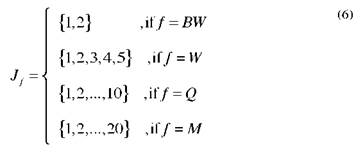
We use the letters L, J and K to denote the sets of customers, days, and clusters; F = {M, BM, W, BW} is the set of visit frequencies, where M is monthly, BM bimonthly, W weekly, and BW biweekly. Each customer l ∈ L has a defined visit frequency f G F and a set C f of allowable combinations of visit days associated with the frequency f. L f is the set of customers with frequency f, and V l , is the coordinate vector of customer l. The problem consists of assigning each customer to one cluster k ∈ K and one allowable combination of visit days c ∈ C F in such a way that the customers visited by the same truck in the same day are as close as possible; the closeness criterion is explained later.
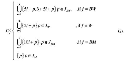
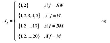
The characteristics of the problem given in Section 1 are as follows: K = {1,2, ..., 9} (nine trucks), /= {1,2, ..., 20} (20 days), and C' is given by equations (1)-(3). For instance, C BM = {{1,11}, {2, 12}, ..., {10,20}} because, as we mentioned in Section 1, the customers with bimonthly frequency must be visited on the first and third Mondays (days 1 and 11) or on the first and third Tuesdays (days 2 and 12), etc.
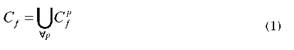
Where
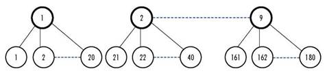
Our general idea for bringing together the clustering and allocation phases lies in the fact that we can represent the customers of each cluster (truck) that are visited in the same day by a sub-cluster. The sub-clusters are denoted by an index n, which depends on the values of j ∈ J and G K, n(j, k) = j + 20(k + 1), that is, one sub-cluster n corresponds to each day and each cluster. In Figure 1, the top circles represent the clusters and the low circles the sub-clusters. Note that each cluster has 20 associated sub-clusters that represent the 20 days of the planning horizon.
The previous transformation forces us to change the set of allowable combination visit days (C ) to a set of allowable sub-cluster combinations C f associated with each frequency. A compact expression for C f is given by equations (4)-(6).
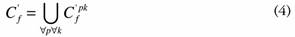
Where
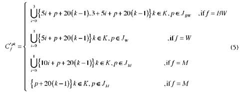
Now we obtain a classical PVRP with one truck, 120 days, and a new set of allowable combinations of visit days C ’ f for each visit frequency f. In creating the sub-clusters, we group the customers by a closeness criterion. A common one is to minimize the sum of the distances of all customers to all of the sub-cluster centroids (C n ) that they belong to. In addition to the variables (C n ), we define the binary variables y k equal to 1 if the allowable sub-cluster combination c S Cfis assigned to customer l and zero otherwise. We use binary constants α nc equal to 1 if sub-cluster n belongs to c ∈ Cf and zero otherwise; the maximum number of customers allowed in each sub-cluster is denoted by w. Because w is minimized, it must be the nearest integer greater than or equal to the average number of customers by sub-cluster.
The model is as follows:
Objective function:
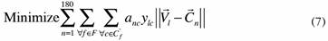
Subject to:
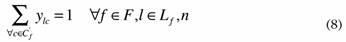
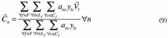
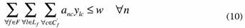

Constraints (8) guarantee that each customer is assigned to one allowable combination of sub-clusters. Constraints (9) are the equations of the sub-cluster centroids, and finally, the role of constraints (10) is to impose a maximum number of customers that belong to each sub-cluster.
The resulting model is non-linear and combinatory, with continuous (C n) and binary variables (y ln ). In the next section, we propose two heuristic approaches for obtaining the solution.
3. Solution approach
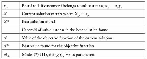
Before presenting the heuristics, additional notation is introduced in Table 1. We drop the variables ylc; instead, we use xln equal to 1 if customer l belongs to sub-cluster n and zero otherwise. An important feature of model (7)-(11) is that it becomes an integer linear program (ILP) if the variables (C n) are fixed as parameters. This modified model is denoted by Mfix .
3.1. Heuristic 1
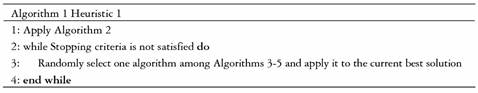
Heuristic 1 (Algorithm 1), includes four sub-heuristics; the first one (Algorithm 2) builds an initial solution, while the others (Algorithms 3-5) try to improve the solutions obtained.
3.1.1. Constructive heuristic (Algorithm 2)
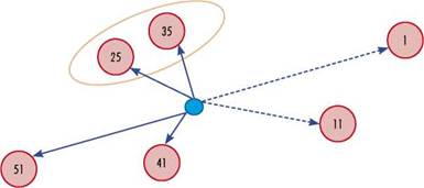
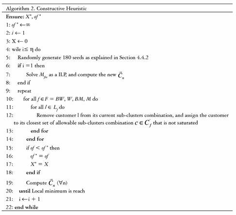
The core of the constructive heuristic (Algorithm 2) is to assign each customer to its closest c ∈ C f that is not saturated, where closest means that the average distance to all sub-clusters n ∈ c is minimum, and saturated means that at least one n ∈ c already has w customers. A graphical example of this procedure is given in Figure 2, where the red circles represent the sub-cluster centroids, and the blue circle is a customer l G L BM . Suppose that pairs {1,11}, {25,35} and {41,51} are the only c ∈ C ’ BM that are not saturated. Therefore, the customer is assigned to c = {25,35} because, on average, the customer is closer to n = 25 and n = 35 than to the other two pairs. Regarding the algorithm’s structure, the inner while loop performs the previous procedure, calculates the new centroids, and repeats these two steps interactively. The outer while loop explores other regions in the solution space by randomly restarting all centroids. Note that in the first iteration of the outer while loop, Mfix is solved. The purpose of this is to ensure that the algorithm starts from a feasible solution.
3.1.2. Improvement heuristics
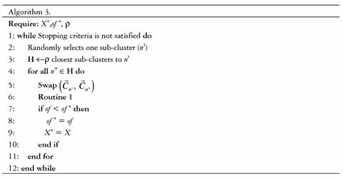
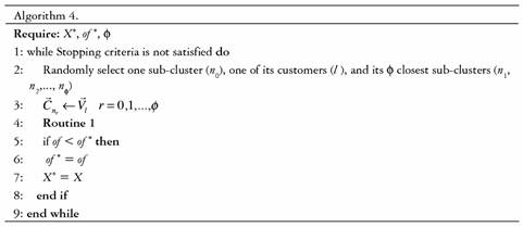
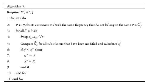
Algorithms 3-4 are shaking procedures, with the common idea of making changes in the coordinates of one or several centroids, followed by performing the same routine as the inner while loop of Algorithm 2, henceforth referred to as Routine 1. Algorithm 3 selects one sub-cluster randomly (n’) and sets up the vector H with its closest sub-clusters, where the closeness criterion is the distance between the sub-cluster centroids. Then, one sub-cluster n' ∈ H is taken, and the coordinates of the centroids of n and n” are swapped, followed by Routine 1. Algorithm 4 selects one sub-cluster randomly (n0) and one of its customers and changes the centroid's coordinates of n Q and its Φ closest sub-clusters for the selected customer coordinates, followed again by Routine 1. Finally Algorithm 5 is a local search that swaps the assigned sub-cluster combination between two customers that have the same visit frequency.
3.2. Heuristic 2
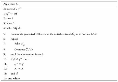
The second solution method (Algorithm 6) is an adaptation of the heuristic presented in [12], with m any more binary variables, as it considers all the customers of the company to be visited. The algorithm starts by randomly selecting 180 initial seeds as centroids C n and solving the resulting M fix using adequate software, in our case, Gurobi with AMPL. With the solution, the new centroids are calculated, and a new M fix is solved. These two steps are repeated interactively until a local minimum is reached (we consider that the local minimum is reached if the best solution has not improved more than 0.05%). When the local minimum is reached, new random initial seeds are generated in order to explore other regions in the solution space.
4. Computational experiments
4.1. Test instances
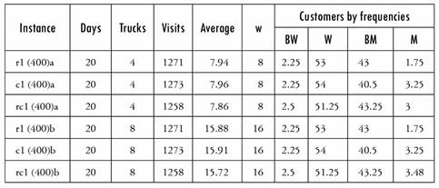
A set of instances from [13] are considered, taking into account the characteristics of the company. The instances are differentiated by two main criteria: first, the geographical distribution of the customers in R2, where class r is those where the customers are uniformly distributed, class c those with dense clusters of customers, and rc a combination of r and c; second, the different frequencies of distribution relative to the total number of customers, which are denoted by 1, 2 and 3.
We use the notation r*, c* and rc* when we refer to instances of type r, c and rc with any of the different frequency types of distribution (1, 2 or 3). Analogously, *1, *2 and *3 are associated with instances with specific frequencies of distribution (1, 2 or 3), regardless of the configuration of customers with regard to their geographical distribution (r, c or rc).
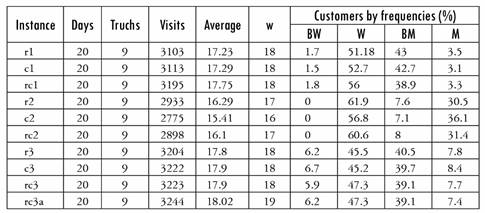
Instances of type *1 have the lowest percentage of customers with monthly frequencies compared to the other two types of distributions, with an intermediate percentage of customers with biweekly and weekly frequency compared to the other two types of distributions. Instances of type *2 do not have customers with biweekly frequencies and have the highest percentage of customers with monthly and weekly frequencies and the lowest percentage of customers with bimonthly frequencies compared to the other two types of distributions; the most significant differences are in monthly distributions. Instances of type * 3 have the highest percentage of customers with biweekly frequencies compared to the other two types of distributions. These characteristics are shown in Table 2. The last row of Table 2 shows one type of instance (rc3a) very similar to instance rc3. It is constructed from rc3 by changing the visit frequency of 3 customers from monthly to bi-weekly. The number of total visits to be made increases, but the gap of the average of visits to the nearest smaller integer increases.
4.2. Parameter settings, stopping criteria and run times
4.2.1. Heuristic 1
The algorithm’s parameters must be adjusted in consideration of the size of the instance. In our tested instances, we found efficient results for η = 100, p = 8, Φ = 6, γ = 5.
Regarding the stopping criteria for Algorithm 1, we found that repeating line 3 eight times was sufficient; above this value, we did not obtain a significant improvement in the solution in contrast to the time spent, while Algorithms 3-4 stop if the objective function has not improved at least 0.05% within 50 seconds. With this configuration, we ran Algorithm 2 10 times for all instances. The algorithm was coded in MATLAB with an average run time of15 minutes.
4.2.2. Heuristic 2
To make the times comparable between both heuristics, we report the results when setting η’ = 80, although it does not provide considerably better results that those obtained with a lower η’. This is shown in Table 4.
4.3. Numerical Results
Table 3 reports the results obtained for each of the instances. In column 2, the best value of the Hybrid Heuristic, in column 3, the best value of Heuristic 1, and in columns 4 and 5, the average and standard deviation with respect to the solutions of Heuristic 1 are shown. Columns 6 to 8 show the results of Heuristic 2. The last column reflects the gap in the average values obtained by both Heuristics 1 and 2.
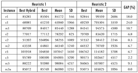
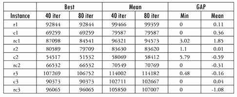
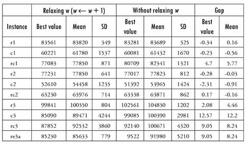
Table 5 reports the results of the Hybrid Heuristic when relaxing w (w - w + 1) during Heuristic 2 and then solving Mfix with the original w, compared with the results without relaxing w. The relaxation is done to increase the possible movements of Heuristic 1, as the heuristic can make more changes to the solution, especially in instances * 3, where the average is closer to w than in the other instances.
4.4. Sensitivity analysis
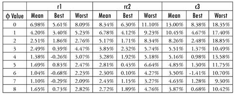
4.4.1. Parameters ρ, Φ, γ
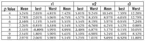
To analyze the importance of the values of p and f, we test different values of these parameters by running Algorithm 1 solely with Algorithm 3 or 4 as improvement procedures. For this purpose, we choose instances r1, rc2 and c3, which provide different characteristics regarding the geographical position of the customers and the percentage of customers with each frequency. In Tables 6 and 7, we report the best, average and worst deviations from the best results of Heuristic 1 in Table 3 over 10 runs. The parameter y is just to speed up the algorithm, because there might be some customers that are too far from each other, and it is not worth doing a permutation with them. We found no typical behavior in the results of Table 6; nevertheless, p = 8 is the best value in general. Conversely, f shows the best results when set equal to 6.
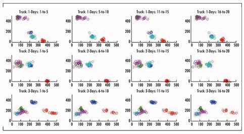
4.4.2. Initial seeds
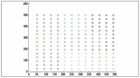
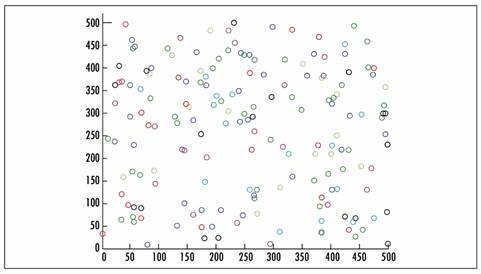
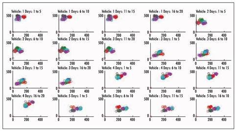
The initial seed location has proven to have an important role in the final results. In Figure 3, we show our initial arrangement where the 20 initial seeds for each truck are placed close to each other. In Figure 4, the 20 initial seeds for each truck are randomly spread over all regions. The final results of both initial arrangements are shown in Figs. 5 and 6, where the customers assigned to the same day are marked in the same color (for a better visualization, we just show the assignation for trucks 1 to 5). The results are more visually appealing, and the objective function is usually 5% to 10% better. Even though the creation of the routes is not part of the scope of this work, initial experiments have shown lower route costs when the seeds are arrange as in Figure 3.
4-5. Computational times
We now present a computational time analysis, introducing some new instances in Table 8. We reduce the number of customers to 400 and the number of trucks to 4 and 8.
5. Discussion
Comparing instances of types * 1, * 2 and * 3, Table 3 shows that taking into account both the best value found and the average of the values of the objective function, they increase in the order c, rc, and r, according to the geographical distribution of customers. The standard deviation (SD) generally has no typical behavior. These results seem logical for the types of distribution of the points and their possible proximity to the associated centroids. A significant exception is found when comparing the results of Heuristic 1 (also Hybrid) with the instances of type * 3, which increase in the order rc, c, and r. However, with other instances similar to those of type * 3, the trend seen in the other examples is reflected.
Comparing the instances of types r *, c * and rc *, Table 3 also shows that for all algorithms implemented, taking into account both the best value found and the average value, the values of the objective function increase in the order 2, 1, and 3 of the frequency distribution. The SD generally behaves in the same way. This could be in relation to the total number of visits to be made, which decreases in the same order.
5.1. Algorithm performance
The best results are obtained by the Hybrid Heuristic when relaxing the upper bound (w - w + 1) during the Heuristic 2 phase. Because Heuristic 2 performs better if most of the clusters are not saturated, the algorithm moves more freely through the solution space. Experiments show that if w is too close to the average of customers by sub-cluster, worse results are obtained even though the number of visits may increase, such as in the case of instances rc3 and rc3a.
It is important to note that if all the customers have a monthly frequency of visits and
W ← ∞, both Algorithms 2 and 6 perform as k-means algorithms [23].
Heuristic 2 is the repetition for a given number of iterations of a solver of a mixed integer linear programming (MILP) problem with binary variables (greater percentage) and continuous variables. The solution time depends mainly on the number of binary variables. The binary variables depend on the number of customers and the number of trucks (clusters). When one of these two parameters increases, the size of each MILP problem increases, and the number of binary variables and the solution time of each iteration increase. For example, in the computational experiments carried out, when varying the number of clients from 400 to 1 000 and keeping the remaining parameters fixed, the average time in the solution of each MILP problem varies from 0.02 to 0.05 seconds.
In the same way, setting the number of customers at 1000 and varying the number of trucks from 4 to 9, the average time for the solution of each MILP problem varies from 0.05 to 0.107 seconds. In relation to Heuristic 1 and its execution time, the results are given in Table 10.
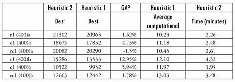
Table 10 Solution times for Heuristic 1 for different numbers of customers and trucks
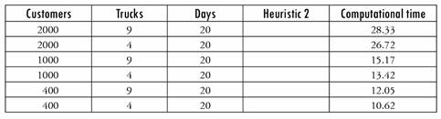
Source: Author's own elaboration
In terms of solution quality, by increasing the number of trucks and maintaining the same number of customers, it is logical that the solution improves in both heuristics, decreasing the value obtained from the objective function (Table 9).
5.2. Balancing workload
The model (7)-(11) does not have a lower bound for the number of customers belonging to the sub-clusters; this means that it could be the case that no customer is assigned to a particular sub-cluster. If a more balanced workload among all routes is desired, a lower bound can be introduced into the model. The solution approaches do not change much, for instance, the Hybrid Heuristic can be applied by letting Heuristic 1 remain as is and, at the end, solving Mfix with the lower bound additional constraint. If the average of customers per sub-cluster is very close to w, this balance is automatic.
6. Conclusions and future work
We presented novel solution approaches to assign customers to trucks and days in a PVRP like problem with the additional constraint that every customer must always be visited by the same truck.
Our method is very useful for instances with a great number of allowable combinations of visit days. The generalization for capacity constraints in the daily routes is straight forward and can be done in all Heuristics with w equal to the maximum capacity.
Future work consists of the creation of routes for each sub-cluster that correspond to a problem of type TSP (traveling salesman problem), which can be solved by a simple insertion heuristic and further improvements in the solutions with local search procedures and meta-heuristics.

