Modelación de la concentración atmosférica de CO usando regresión no paramétrica con bandas de variabilidad no homogéneas

CO atmospheric concentration modeling using nonparametric regression with non-homogeneous variability bands

Alvaro J. Flórez
Statistics school, Universidad del Valle, Cali, Colombia
E-mail: alvaro.florez@correounivalle.edu.co

Eje temático: Ingeniería ambiental, Estadística / Enviromental engineering, stadistics
Recibido: 7 de Marzo de 2013
Aceptado: 30 de Septiembre de 2013

Resumen

La contaminación del aire por monóxido de carbono (CO) es uno de los principales factores que afecta la calidad del aire en las grandes ciudades, pues está directamente relacionado con las actividades urbanas. El comportamiento medio y de la variabilidad de las concentraciones de CO a lo largo de un día varía constantemente debido principalmente al tráfico vehicular en el lugar. El objetivo de este trabajo es proponer un modelo de suavización no paramétrico para la concentración horaria de CO en el aire, considerando varianza no constante, que permita describir su comportamiento a lo largo de un día. Para esto se usaron los registros de contaminación por CO en una estación ubicada en el centro de la ciudad de Cali, Colombia. Se estimaron las curvas por medio de regresión lineal local y la función de varianza por medio de un estimador de la función de varianza. Las curvas estimadas permitieron describir el comportamiento del CO, mostrando mayores concentraciones en horas "pico" y menores en la madrugada, además la estimación de una función de varianza permitió modelar de mejor forma el comportamiento heterocedástico de los datos.

Palabras claves: contaminación atmosférica, estimadores basados en diferencias, monóxido de carbono, regresión no paramétrica.

Abstract

Air contamination by carbon monoxide (CO) is one of the main factors affecting the air quality in big cities, since it's directly related to urban activities. The CO concentrations variability average behavior changes constantly mainly due to the traffic in the place. The objective of this article is to propose a non-parametric smoothing model for the hourly CO concentration in the air, considering non-constant variance that allows the description of its behavior through the day. To this end, contamination records by CO in a downtown pollution monitoring station in Cali, Colombia were used. Curves were estimated by using local lineal regression and variance function through an estimator of variance function. The estimated curves allowed describing the CO behavior, showing bigger concentrations in rush hours and smaller concentrations in the early morning, besides the variance function estimation allowed to better model the data's heteroscedastic behavior.

Keywords: atmospheric contamination, carbon monoxide, difference-based estimators, non-parametric regression.

1. Introduction

The development going on since the 20th century has notoriously changed the demographic characteristics of Latin American population, so that nowadays more than 70% of these countries population is located in urban areas, and in Colombia most of the urban population is concentrated in four main cities (Jaramillo et al., 2009). Because of this, the industrial and economic activities and the constant vehicles circulation have increased rapidly in urban centers, in some cases, without a good planning in environmental terms, which creates in the end, harmful effects to the environment that affect life quality of the citizens (Romieu et al, 1991).

Air pollution in the cities, that it is a product of human activities, has a negative impact on people's health, these effects go from short time effects such as eye and nose irritation and sore throat to chronic respiratory diseases (Xia & Tong, 2006). These consequences can be worse on people with chronic diseases, children and the elderly. Amongst all of the contaminants that can be found in a city we find CO, which is produced by the incomplete combustion of hydrocarbons, being the emissions from vehicles' exhausts the main source in urban areas (Georgoulis et al, 2002). Due to this CO's behavior is highly determined by vehicle's circulation and industrial activities. According to Samoili et al (2007) CO concentration shows a spatially heterogeneous behavior in a city, but its biggest concentrations appear in places with high volume of traffic.

Due to the fact that CO concentration is highly related to urban activities, it is important to study how its behavior is throughout the day, since high values are expected to show up when there is high activity, for instance, in rush hours when the volume of traffic is higher. Reina & Olaya (2012) and Montoya et al (2005) have shown that the non-parametric regression techniques, such as spline or local regression, are appropriate to modeling the daily behavior of contaminants and are also useful in the decision making about air quality, emphasizing the use of variability bands to the comparison of different estimated curves for contaminants. However, to use these bands it is necessary to estimate the variance in the contaminant concentration for each hour of the day; generally this is assumed as constant and one of the estimators proposed in literature is used (Rice 1984; Gasser et al, 1986; Hall et al, 1990). But the hourly behavior of CO does not seem to adjust to this assumption, since the variability measures seem to be higher when there is a higher human activity and vice versa. In these cases the use of alternative techniques for the use of variability bands is necessary.

Taking into account the negative effects of this contaminant over the population, a tool to understand its behavior throughout the day becomes relevant, this would allow to take control and prevention measures. Therefore the main purpose of this paper is to propose a nonparametric model for the hourly behavior of the CO concentrations using non-homogeneous variability bands, using the variance estimator proposed by Brown & Levine (2007). In order to illustrate this model the CO hourly measuring records from 2004 in a pollution monitoring station located in downtown Cali, Colombia (station named CALLE15) were used. This station is one of interest due to its location on a zone of high commercial activity, besides a high volume of traffic and pedestrian activity. The data used for this was provided by the Red de Monitoreo de la Calidad del Aire (RMCA) of DAGMA, which in 2006 had 8 fixed stations located in different sectors of the city. From 2010 on the RMCA restarted operations, but only with 2 fixed stations located in the north of the city.

2. Methodology

2.1 Non-parametric regression model

Härdle (1990) suggests that non-parametric regression has as an objective to adjust a regression curve that describes the relation between the variables x_i and y_i, where is considered that x_i explains the value of y_i. If n observations appear (x_i, y_i), the regression curve is commonly modeled as:

Where ε is a random variable that indicates the variation of Y around m(x), that represents the mean of the regression curve E (Y|X = x). Besides it has to be assumed that ε_i have E(ε_i) = 0 and var(ε_i) = σ² < ∞.

In the framework of non-parametric regression estimations through variability bands can be made, these are equivalent to the confidence intervals in parametric regression, where it's necessary to have variance estimation. In literature several variance estimators can be found, such as the estimators based on differences proposed by Rice (1984), Gasser et al (1986) and Hall et al (1990). In some cases it's not possible to assume that the variance of ε_i is constant, but that it depends on the independent variable (x_i), because of this a variance estimation different from the above mentioned would be needed. For the estimation of a heteroscedastic model in Brown & Levine (2007) the regression model is set in this way:

And a variance function estimation f(x) through a smoothing that reflects the variability of m(x) in function of x is proposed.

2.2 Estimation of the regression curve

As mentioned in Olaya (2012) the goals of the analysis of the non-parametric regression are the same than its parametric counterpart. It's valid to say, estimate and prove the characteristics of the regression function. The procedure to estimate the regression function m in model (1) in the framework of non-parametric regression is called smoothing.

To use smoothing techniques, unlike parametric regression techniques that possess several assumptions in the model, it's only necessary to assume that m is smooth, which could say that for the curve adjustment in a determined point of x, is expected that observations y_i associated to x_i near x, possess information of m in the interest point of x (Eubank, 1999). For the function to be smooth it must be considered that m belongs to a space of functions W, where W is assumed as the group of all functions m that have k continuous derivatives in (a,b) (Olaya, 2012).

This said, these methods make a weighted average of y_i depending on the distance of x_i, where the most common smoothers are the linear estimators that look like:

Where K (x, x_i; λ) is a collection of weights that depend on the smoothing technique, the distance between points {x_i; i = 1, 2,... , n}, point x of estimation and of a λ > 0 called smoothing parameter, in charge of determine the smoothing degree to the data. Therefore λ is the only parameter necessary to be estimated for the adjustment of the curve.

One of the most used linear estimators is the local average estimator or Nadayara-Watson, which is a modification of (3) where it's assured that the addition of weights equals one. This estimator is defined as:

Where K is a Kernel function that is in charge of assigning weight to the observations near the point of estimation x, with the characteristic that the weights of this estimator do not depend on the group of values X that intervene in the estimation.

Another choice for the construction of the data local average is to adjust a local linear regression (Azzalini & Bowman, 1997), as shown in (5).

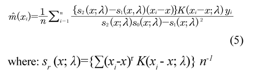
Same as estimator (4), the objective of weight function K is to guarantee that the observations near x have a bigger weight on the estimations. Fan & Gijbels (1996) show the excellent theoretical properties of this estimator. In particular, the estimations near to the boundaries through local linear regression are superior than the ones through local average.

The smoothing parameter λ determines the width of the Kernel function, therefore, if λ is small, the estimations will be close to the observed values, a small bias, but acquiring a high variability. Otherwise, the estimation will be too smooth, reducing the bias, but the variance would increase (Azzalini & Bowman, 1997). Taking this into account, the selection of an optimal λ becomes important in the adjustment of the estimated curve.

Cross validation is the most used method for the selection of the smoothing parameter (Azzalini & Bowman, 1997), which consists in finding a λ that reduces the mean quadratic error of m(x_i). This method is based on the prediction of the answer in point x_i through the adjustment of the curve with the remaining observations{x_j, y_j}, i ≠ j. Taking that into account the cross validation function is defined as:

For a point x_i, its prediction is denoted as m_-i(x_i), where the sub index -i indicates that observation (x_i, y_i) was omitted . Therefore the cross validation method consists of finding the value of λ that makes function (6) minimum.

2.3 Variability bands

In any statistics modeling the representation of the estimated curve through confidence intervals is of great usefulness, since these indicate the degree of uncertainty associated to the estimation of m(x). One of the assumptions made while forming confidence intervals is that errors are normally distributed, in which case the confidence interval can be made through the following pivotal quantity:

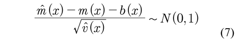
Where v̂ (x) indicates the variance of m̂ (x) and b(x) indicates the estimation bias. The inconvenience resides in the fact that the estimation of b(x) could become a complex problem (Azzalini & Bowman 1997).

One alternative is the use of variability bands, these can be used as an indicator of the variability level involved in the non-parametric estimation without attempting to adjust for the inevitable presence of bias (Azzalini & Bowman 1997). The difference with the confidence intervals is that the bands indicate pointwise confidence intervals for E(m̂ (x)) instead of m(x), therefore one must be careful with the interpretations. Taking that into account, they can be formed by indicating the size of two standard errors above and below the estimation. Where it would have a variability estimation of m̂ (x).

2.4 Estimation of the variance

Due to the estimations of m(x) are biased, in the non-parametric context there is a considerable number of estimators of σ², where the differencebased estimators that use yi responses associated to a predetermined neighborhood of x, are the most used since these have the advantage of not depending explicitly of the smoothing technique that is being used (the order of the differences is determined by the number of successive observations used for the calculations of the local pseudo-residual). These types of estimators are presented in a general way by Gasser et al (1986) and Hall et al (1990).

Brown & Levine (2007) do not suggest a point variance estimation, instead they suggest the estimation of a variance function, in order to do that, consider the model suggested in (2).

Where it's assumed that the errors ϵ_i are independent and identically distributed N(0,σ²), it is assumed for convenience that the design is fixed. The main idea is that the variance does not follow a necessarily constant behavior for all x, but this is ruled by an unknown function f(x_i) and the purpose is to estimate it in the presence of m(x).

Brown & Levine (2007) propose that the variance function can be estimated as a weighted local average of the square of the pseudo residuals of the order r. Where each pseudo residual is a normalized difference of the observations r + 1, defined as:

Where the differences {d_j} satisfy the conditions Σ^r-1_j=0 d_j=0 and Σ^r-1_j=0 d²_j=1. Hall et al (1990) present several alternatives to the section of values {d_j}.

Based on the pseudo residuals, the estimator of the variance curve ˆƒ_h(x) is defined as the smoothing of Δ²r,i:

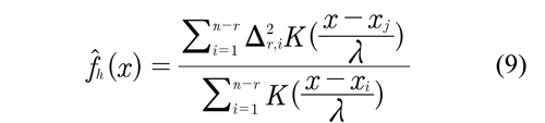
Where λ is the bandwidth proposed and K is a Kernel function. Therefore the pseudo residuals' squares are defined and then locally smoothed in order to produce a Kernel estimation of the variance. Given that Δ²_r,i are not independent; this estimator is not equivalent to the Nadayara-Watson estimator.

3. Results and discussion

3.1 Descriptive statistics

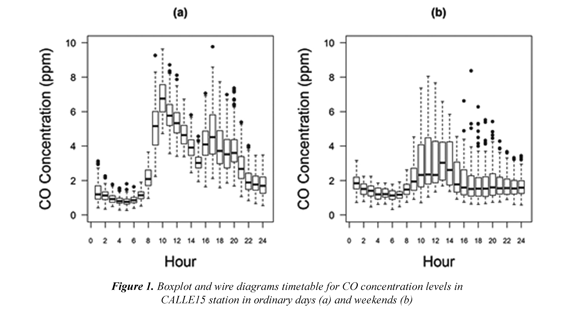
In order to know the behavior of the hourly CO concentration throughout an ordinary day, Figure 1 shows through a boxplot the contaminant for each hour of the day in ordinary days (Monday through Friday) and non-ordinary days (Saturday, Sunday and holidays). It can be appreciated that the CO behavior during ordinary days have its maximum level of concentration around 8 am, at this time it starts descending until approximately 4 pm where another peak appears and later on the observations drop to the minimum in the early morning period, between 0 hours and 6 am. During non-ordinary days the levels of the contaminant show lesser magnitudes, noticing a maximum peak between 10 am and 12 pm. Besides this average behavior it is noticed that the CO distributions for every hour, present different dispersions, very spread distributions in rush hours and only a small dispersion in the early mornings, which can suggest a heteroscedastic behavior.

3.2 Regression curve

The variance function estimation for both ordinary days and non-ordinary days is made through the smoothing of the squared pseudoresiduals, using the local linear regression estimator (5) and a bandwidth estimated by cross validation (λ = 0.313) which are expected to show the heteroscedasticity of the data. In Figure 2 the behavior of the pseudo-residuals can be appreciated for the data in both types of days, where it is clear that for ordinary days the higher values are between 7 am and 9 am, the hours of higher dispersion in CO concentration, while the smooth curve presents lesser values during the early morning, which is expected since at that time we found the lowest dispersion. For non-ordinary days a similar behavior can be found although in lesser magnitude. Taking this into account, the smooth curve of the squared pseudo residuals satisfactorily represents the variance behavior for the hourly CO concentration throughout the day.

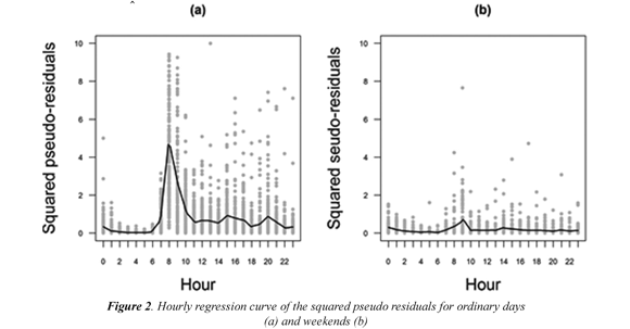
Figure 3 presents the daily estimation of the typical curves for both types of days using the local linear regression estimator (5) and a bandwidth estimated by cross validation (λ = 0.313). The estimated curve for ordinary days shows the mean behavior of the hourly CO contamination, with maximum concentrations around 8 am and a lesser peak around 5 pm, besides the minimum values during the early morning. In non-ordinary days the estimations present much lesser values, although a peak can be appreciated around 9 am. These graphics also show the variability bands for the estimation, taking into account the estimated variability function which presents as well wide bands in hours when data variability is higher and short bands when the dispersion is low. For comparison effects the bands for the case where the variance is supposed as constant is presented, making evident that the bands are unnecessarily big during the hours with less variability and too small on the opposite case, altering the proposed confidence level.

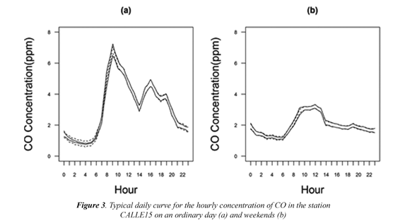
Cyclical behaviors of CO concentrations during an ordinary day, where two maximums are noticed throughout the day and the lesser magnitude curves for non-ordinary days, are coherent with the hypothesis that says that vehicles circulation and human activities are the main causes of high level of pollution. It could be noticed that during rush hours -when the traffic volume is higher- the biggest measures for CO appeared. Besides on weekends when there's less commercial activity in downtown the curves had lesser levels.

It was noticed that CO distributions for each hour have different variability; therefore Brown & Levine (2007) proposal for the estimation of the variance function was accurate. This estimation represented in a more realistic way the heteroscedastic behavior of the variable. This is reflected in the estimated variability bands, since they show higher variability in hours when the dispersion was higher and vice versa. The use of bands assuming constant variance could lead to erroneous conclusions since it would be altering their confidence level.

4. Conclusions

Taking into account that the negative impact on people's health depends on exposure time and the contaminants concentration (Samoli et al, 2007). The estimated curves are of great importance to the entities in charge of controlling the quality of air, since they can be used to generate policies for the reduction of pollution levels, especially during hours when the levels are at maximum.

The use of a model that allows the modeling of contaminants concentrations in the air during an ordinary day will act as a supply so the entities in charge of health can promote epidemiology studies that determine the impact that the exposure to the contaminants has on health, particularly on the population that is exposed during long periods of time on hours where the concentration is higher. According to the negative effects and the estimated curves of the hourly concentration of contaminants, preventive measures can be created for the population of higher exposure in these places.

Non-parametric regression methods and the variance function estimator used are useful tools for the modeling of the daily behavior of the contaminants concentration. For these contaminants show very variable behaviors in the average and variance which makes difficult the use of a parametric technique.

The introduced model although it models the heteroscedastic behavior of the hourly concentration of CO, does not take into account other atmospheric and climatological factors that could alter the regular behavior of the contaminants, such as temperature, wind speed or precipitation (Reina & Olaya, 2012; Montoya et al, 2005). Therefore the use of generalized additive models (GAM) (Hastie & Tibshirani, 1990) is recommended, these allow the introduction of these covariates in the nonparametric model and this way obtain a model that can better describe the contaminants behavior.

One aspect to take into account is the temporary correlation that the data could show, since this alters the bandwidth selection through cross validation, giving values of λ that can over smooth the curve estimation (giving biased estimations) if there is a negative correlation, or leads to a interpolation of the data (high variability estimations) if the correlation is positive. For this, several authors (Altman, 1990; Hart, 1991; Opsomer et al 2001) have proposed a series of bandwidth selectors based on the structure of data correlation.

The same correlation problem appears for the estimation of the variance function. An alternative proposed by Brown & Levine (2007) is the use of the cross validation k-fold, which is not based on the prediction of each observation through the adjustment of the curve with the remaining observations, but on the prediction in k groups of observations.

Although non-parametric regression models were a satisfactory way for the modeling of this contaminant, the functional data analysis (Ramsay & Silverman, 2005) could also be used, since on data structure the hourly observations of each day could be treated as functional data for its modeling.

5. References

Altman, N. (1990). Kernel smoothing of data with correlated errors. Journal of the American Statistical Association , 85 (411), 749-759.         [ Links ]

Azzalini, A., & Bowman, A. (1997). Applied smoothing techniques for data analysis. Oxford, UK: Oxford University Press Inc.         [ Links ]

Brown, L., & Levine, M. (2007). Variance estimation in nonparametric regression via the difference sequence method. Annals of Statistics , 35 (5), 2219-2232.         [ Links ]

Eubank, R. (1999). Nonparametric regression and spline smoothing. New York: Marcel Dekker.         [ Links ]

Fan, J., & Gijbels, I. (1996). Local Polynomial Modelling and Its Applications. London, UK: Chapman & Hall.         [ Links ]

Gasser, T., Sroka, L., & Jennen-Steinmetz, C. (1986). Residual Variance and Residual Pattern in Nonlinear Regression. Biometrika , 73(3), 625-633.         [ Links ]

Georgoulis, L., Hänninen, O., Samoli, E., Katsouyanni, K., Künzli, N., Polanska, L., et al. (2002). Personal carbon monoxide exposure in five European cities and its determinants. Atmospheric Environment , 36 (6), 963-974.         [ Links ]

Hall, P., Kay, J. W., & Titterington, D. M. (1990). Asymptotically Optimal Difference-Based Estimation of Variance in Nonparametric Regression. Biometrika , 77 (3), 521-528.         [ Links ]

Härdle, W. (1990). Applied Nonparametric Regression. Cambridge, UK: Cambridge University Press.         [ Links ]

Hart, J. (1991). Kernel regression estimation with time series errors. Journal of the Royal Statistical Society , 53(1), 173-187.         [ Links ]

Hastie, T., & Tibshirani, R. (1990). Generalized Additive Models. New York: Chapman and Hall.         [ Links ]

Jaramillo, C., Ríos, P., & Ortiz, A. (2009). Incremento del parque automotor y su influencia en la congestión de las principales ciudades colombianas. 12do encuentro de geógrafos de América Latina. Montevideo, Uruguay.         [ Links ]

Montoya, M., Morales, A., & Olaya, J. (2005). Estimación no-paramétrica de curvas típicas diarias para los contaminantes CO, NO2 y SO2 en Santiago de Cali. Revista Ingenieria de Recursos Naturales y Del Ambiente , 2 (1), 23-27.         [ Links ]

Olaya, J. (2012). Métodos de regresión no paramétrica. Cali, Colombia: Programa Editorial Universidad del Valle.         [ Links ]

Opsomer, J., Wang, Y., & Yang, Y. (2001). Nonparametric regression with correlated errors. Statistical Science , 6 (2), 134-153.         [ Links ]

Ramsay, J., & Silverman, B. (2005). Functional Data Analysis. London: Springer.         [ Links ]

Reina, J., & Olaya, J. (2012). Ajuste de curvas mediante métodos no paramétricos para estudiar el comportamiento de contaminación del aire por material particulado PM10. Revista EIA , 18, 19-31.         [ Links ]

Rice, J. (1984). Bandwidth choice for nonparametric kernel regression. The annals of Statistics , 12 (4), 1215-1230.         [ Links ]

Romieu, I., Weitzenfeld, H., & Finkelman, J. (1991). Urban Air Polllution in Latin American and the Caribbean. Journal of the Air & Waste Management Association , 41 (9), 1166-1171.         [ Links ]

Samoli, E., Touloumi, G., Schwartz, J., Anderson, H., Schinder, C., Forsberg, B., et al. (2007). Short-Term Effects of Carbon Monoxide on Mortality: An Analysis within the APHEA Project. Environmental Health Perspectives , 115 (11), 1578-1583.         [ Links ]

Wang, L., Brown, L., Cai, T., & Levine, M. (2008). Effect of mean on variance function estimation in nonparametric regression. Annals of Statistics , 36 (2), 646-664.         [ Links ]

Xia, Y., & Tong, H. (2006). Cumulative effects of air pollution on public health. Statistics in Medicine , 25 (20), 3548-3559.         [ Links ]

Revista Ingeniería y Competitividad por Universidad del Valle se encuentra bajo una licencia Creative Commons Reconocimiento - Debe reconocer adecuadamente la autoría, proporcionar un enlace a la licencia e indicar si se han realizado cambios. Puede hacerlo de cualquier manera razonable, pero no de una manera que sugiera que tiene el apoyo del licenciador o lo recibe por el uso que hace.