A unified integral interpretation of thermal analysis data

Una interpretación integral unificada de los datos de análisis térmico

J. I. Carrero-Mantilla
Chemical Engineering Department, Universidad Nacional de Colombia. Manizales, Colombia.
E-mail: jicarrerom@unal.edu.co

A. F. Rojas-González
Chemical Engineering Department, Universidad Nacional de Colombia. Manizales, Colombia.
E-mail: anfrojasgo@unal.edu.co

J. M. Cárdenas-Giraldo
Chemical Engineering Department, Universidad Nacional de Colombia. Manizales, Colombia.
E-mail: jumcardenasgi@unal.edu.co

Eje temático: CHEMICAL ENGINEERING / INGENIERÍA QUÍMICA
Recibido: Junio 11 de 2015
Aceptado: Septiembre 17 de 2015

Abstract

Most integral methods for thermal analysis data use linear regressions based on some approximate representation of the temperature integral. But this approach is inconvenient because there are many approximations and each one can produce a different result for the same data set. This work shows how to reduce the search of kinetic parameters to a non-linear regression calculating the temperature integral through the incomplete gamma function. In this way the use of approximations is avoided and dependence of the preexponential factor on temperature can be included in the model. An isoconversional analysis of a data set available in the literature is used to explain the proposed method.

Keywords: Incomplete gamma function, non-linear regression, temperature integral, thermogravimetric analysis.

Resumen

La mayoría de los métodos integrales para el análisis de datos térmicos utilizan regresiones lineales, basadas en alguna representación aproximada de la temperatura integral. Pero este enfoque es inconveniente porque hay muchas aproximaciones distintas y cada una puede producir un resultado diferente para el mismo conjunto de datos. Este trabajo muestra cómo reducir la búsqueda de parámetros cinéticos a una regresión no lineal calculando la integral de temperatura con la función gama incompleta. De esta forma se evita el uso de aproximaciones, y se puede incluir en el modelo la dependencia del factor preexponencial respecto a la temperatura. Se usó un análisis isoconversional de un conjunto de datos disponible en la literatura para explicar el método propuesto.

Palabras clave: Análisis termogravimétrico, función gama incompleta, integral de temperatura, regresión no lineal.

1. Introduction

In thermal analysis by thermogravimetry a sample of material is heated, usually at a constant rate, and its mass (w) and temperature (T) are measured during the heating process. The results of the analysis are T and the fractional extent of conversion, defined as

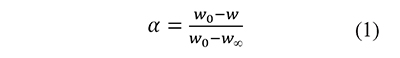
where w₀ and w_∞ are the measurements at the beginning and the end of the analysis, respectively. In the kinetic models used in thermal analysis the variation in time of α is commonly represented as the product of a temperature-dependent rate constant k, and a kinetic function f (Blaine & Kissinger, 2012),

Including a constant heating rate, β=dT⁄dt, and the Arrhenius equation (Arrhenius, 1889)

Eq. 2 becomes (Brown et al., 2000; Vyazovkin, 2000)

where A is the preexponential factor, E the activation energy, and R is the universal gas constant. Temperature and activation energy are represented in a single dimensionless term, x=E⁄RT, and A is usually taken as a constant. The integration of Eq. 4 from the initial condition, x₀ (which corresponds to α=0 at T=T₀), to x gives (Flynn, 1997; Flynn & Wall, 1966)

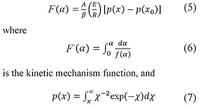
is the temperature integral (or Arrhenius temperature integral). Usually T₀ is the ambient temperature, and p(x₀) is omitted because its value is very small. The argument of the function p(x) is the lower limit of the integral, that is x=E⁄RT, which is different from the running value in the argument of the integral. Therefore, in the integral arguments of Eqs. 7, 8, and 13 the temperature is represented with the symbol τ and the integration variable with χ=E⁄R_τ to emphasize the difference with the limit values.

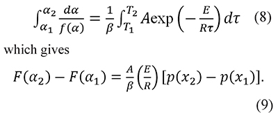
The interpretation of thermal analysis data can also be based on the integration between consecutive α values (Cai & Chen, 2012; Vyazovkin, 2001)

And in some cases the preexponential factor is calculated as a function of the temperature T in the form

where the value of m is an integer or a fraction depending on the reaction or the process (Criado et al., 2005). In this way Eqs. 5 and 9 become

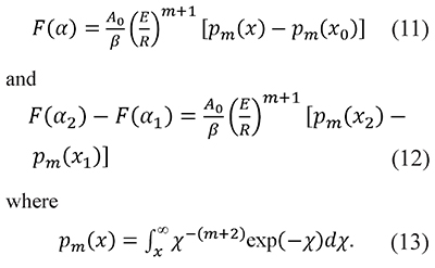
When m=0 Eqs. 7 and 13 are equivalent, i.e. P_m=0(x) = p(x), but we keep different notations Pecause p(x) is a much more common occurrence in chemical kinetics than the general definition Pm(x).

Most proposed integral methods are based on approximations to the function p(x) that reduce the calculation of kinetic parameters to a linear regression problem. For example, the Ozawa-Flynn-Wall method uses the Doyle approximation, log₁₀ p(x)≅ - 2.315 + 0.457x, applied to Eq. 5 to give

where C is a constant (Vyazovkin et al., 2011). The activation energy, E, is obtained from the slope in a linear regression of lnβ vs. 1⁄T data. The approximations to the temperature integral, and the regression methods associated to them, are the subject of several papers due to their widespread application (Aranzazu-Ríos et al., 2013; Jiang et al., 2011; Lyon & Safronava, 2013; Sbirrazzuoli, 2013; Wang & Hsu, 2012; Yunqing, 2014). But the result of such parameter search will depend on the approximation to the temperature integral chosen by the analyst and therefore different sets of A, E parameters can be obtained from the same data. An analyst can compare results from several approximations to select the one that gives the best fit, but it is impossible to include all the approximations that have been proposed in the literature. It makes the data fit uncertain, as there always remain the possibility that another, unknown, approximation gives a better result.

On the other hand a parameter search based on non-linear regression gives a single result: the values of A, E that minimize the difference between observed data and calculated results. Moreover, any kinetic data analysis procedure based on the temperature integral is intrinsically non-linear due to the dependence of x on E. In fact, the non-linear regression interpretation of the integral method appears in the ICTAC (International Confederation for Thermal Analysis and Calorimetry) recommendations, but without a detailed formulation (Vyazovkin et al., 2011). For example, the advanced isoconversional (Vyazovkin-Dollimore) method the activation energy at each conversion, E(α), is calculated through non-linear, one-dimensional minimization (Vyazovkin, 1997). It has been also proposed the calculation of E(α) with iterative search methods, which can be considered equivalent to one-dimensional minimization (Budrugeac, 2010; Budrugeac, 2011; Cai & Chen, 2012). But despite the ICTAC recommendations the non-linear approach is not widely applied and the use of approximations for p(x) appears even in analyses based on non-linear regression.

The prevalence of the linear regression based on approximations to p(x) can be attributed to three reasons. First, non-linear regression seems more difficult because it requires an iterative procedure to minimize an objective function. Second, contrary to linear regression it requires an initial estimate of the result, in this case the kinetic parameters. And third, non-linear regression requires a univocal evaluation of temperature integral, but p(x) does not have analytical solution. All three reasons are questionable: first, in practice the application of non-linear regression is as simple as its linear counterpart because the algorithms are included in modern numerical analysis software. Second, the initial estimates can be typical values found in other analysis, or the result of a complimentary linear regression based on approximations to p(x). And third, there are series representations for p(x), it can be rewritten in terms of special functions, and this integral can be evaluated through numerical quadrature.

A method based on a univocal evaluation of p(x) is more reliable than the use of approximations, but it requires non-linear regression. Therefore this work proposes a unified non-linear interpretation for thermal analysis data based on the search of parameters E, A with non-linear minimization using the incomplete gamma function to evaluate p(x). It is explained first how to cast the search problem in terms of minimization of the differences between calculated and experimental values. The evaluation of temperature integral in terms of exponential integral and incomplete gamma is explained next. Finally, an example based on experimental data is used to show the application of the proposed interpretation. The evaluation of p(x) and Pm(x) with different methods, power series, continued fractions, and numerical integration, is covered in more detail in supplementary material available from the authors.

2. Methods

2.1 Non-linear regression

With a defined F(α) function and taking logarithms Eqs. 5 and 9 become

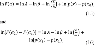
In fact, a similar function was proposed by Cai and Chen for an iterative linear integral isoconversional method (Cai & Chen, 2012). These forms are convenient because the preexponential factor A usually has very high values, therefore the use of ln A prevents the mixture of terms with very different orders of magnitude in the same expression. Then, residuals are defined as the differences between the left-hand and right-hand sides of these equations, i.e.

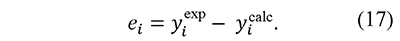
For Eq. 15 .

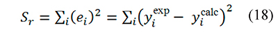
In this way integral-based analysis of thermal decomposition data can be simply described as the search of kinetic parameters ln A, E that minimize the sum of squares of residuals, defined as

Any data fitting regression procedure based on Eqs. 15-18 is intrinsically non-linear because x=E ⁄ RT is a function of the parameter E, and therefore y_i^calc depends on E through the variable x. Given that kinetic data is usually available in the form of α, T measurements made at different β values the integral analysis can be applied in two ways:

non-isoconversional, grouping measure-ments made with the same heating rate β.

isoconversional, with data obtained at the same conversion α.

In the non-isoconversional (single heating rate) variant T(α) data is used to calculate an A,E pair for each β value, but the ICTAC advises not applying it (Brown et al., 2000; Burnham, 2000; Maciejewski, 2000; Roduit, 2000; Vyazovkin, 2000; Vyazovkin et al., 2011). In the isoconversional variant E(α) is calculated grouping the data in sets of T(β) measurements corresponding to the same α value, or consecutive α values (Vyazovkin, 2001). It is not necessary to define in advance the function F(α), and having the result E(α) allows to obtain the time necessary to reach a given conversion (Vyazovkin, 1997). The ICTAC recommends applying isoconversional methods on multi-heating rate data because they produce a reliable mathematical description of the reaction kinetics (Maciejewski, 2000).

Kinetic parameters can be found with isoconversional and non-isoconversional methods using Sr minimization with integration, i.e. using Eq. 15 or Eq. 16. The Vyazovkin-Dollimore method is a different isoconversional approach for E(α) calculation (Vyazovkin, 1997; Vyazovkin, 2001). It is based on the equality of the right sides of Eq. 5 or Eq. 9 at different β values in the forms

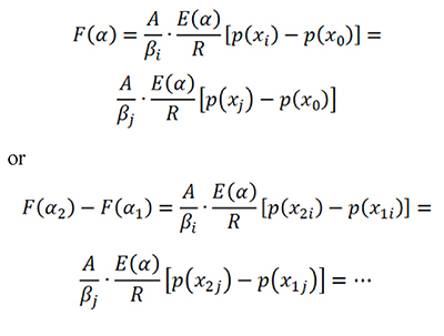
which are grouped in an objective function Φ which is minimized to get E(α). The function based on the integration is

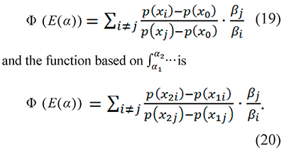
The subscript identifies the heating rate, i.e. x_i=E_i/RT_i where T_i is the temperature measured at the heating rate β_i (the same stands for j). T_1i and T_2i are consecutive temperatures obtained with the same heating rate β_i and x_1i=E_i/RT_1i and x_2i=E_iRT_2i.

Equations 19 and 20 reduce the isoconversional method to a one-dimensional minimization problem: to find, at each α, the E value such that Φ becomes a minimum. An iterative search, the approximation of Φ with a quadratic parabola, and the golden ratio method have been applied to find E(α) (Cai & Chen, 2012; Cai et al., 2010; Vyazovkin, 1997). The minimization procedure is the same when A=A₀T^m but in this case p(x) is replaced with Pm (x), A with A₀, and m is included in Eq. 15 or Eq. 16.

2.2 Calculation of the temperature integral

The integral p(x) has no analytical solution, and the direct use of series representations to calculate p(x) is not practical. But p(x) and p_m(x) can be rewritten in terms of "special functions": the exponential integrals

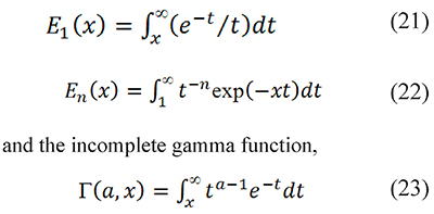
which should not be confused with the standard gamma function (Askey & Roy, 2010). The limitations of series for p(x); and the calculation methods for the functions E1 (x), En (x), and Γ(a,x) are described in the supplementary material available from the authors.

The generalized temperature integral pm(x) defined in Eq. 13 can be calculated with special functions in two ways: replacing t=T⁄τ and x=E⁄RT in Eq. 22

or using the fact that En(x) is a special case of the incomplete gamma function

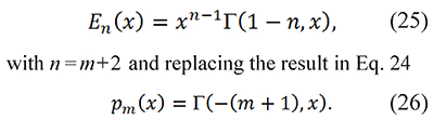
To the best of the knowledge of the authors Eq. 26 is the first proposal to evaluate the generalized temperature integral through the incomplete gamma function. Additionally p(x) can be written in terms of E₁ using integration by parts (Farjas & Roura, 2011)

It can be also calculated making p(x)=p_m=0 (x): with Eq. 24 p(x)=x^-1E2(x), and with Eq. 26 p(x)=Γ(-1,x). The results obtained in this work show that p(x) results are the same with x^-1E2(x) Γ(-1,x), or e^-x⁄x-E₁(x). However, the incomplete gamma function is a more complete way to calculate the temperature integral than the exponential integral because p_m(x)=Γ(-(m+1),x) yielded consistent results (low errors) for any m, integer or non-integer in the interval 1≤x≤100 tested in the supplementary material.

The calculation of temperature integral with numerical integration, with relatively big stepsizes, can be almost as efficient as the application of the incomplete gamma function. But it should be considered that the use of incomplete gamma function does not require to deal with stepsizes or the definition of the upper limit of the integral. Moreover, there are available codes for the calculation of Γ(a,x), and it is implemented in the software Matlab. Therefore we recommend to use p(x)=Γ(-1,x) or pm(x)=Γ(-(m+1),x), and the example in the following section is based on it.

The testing of Eqs. 23, 25, and 26; the details involved in the calculation of E1(x), En (x), and Γ(a,x) , and the comparison of execution times are described in the supplementary material available from the authors.

3. Results and discussion

Kinetic parameters for the decomposition of 2-nitroimino-5-nitro-hexahydro-1,3,5-triazine (NNHT) were obtained from a data set published by (Jiao-Qiang et al., 2009). Following the ICTAC guidelines the analysis was isoconversional, i.e. the parameters were calculated for each α minimizing the functions Sr and Φ. We abstain from comparing results or making statements about the underlying decomposition mechanisms because our proposed method only covers the calculation of the parameters lnA and E, it does not include any further kinetic interpretation.

The NNHT experimental data included temperatures corresponding to 0.025<α<0.975, measured at four heating rates: β= 2, 5, 10, and 15 K/min (Jiao-Qiang et al., 2009). Following the Popescu method two fractional reaction extent values (αa, αb) appearing in the data obtained with all four heating rates were interpolated at T_b=480K and T_a=470K , see Fig. 1 (Popescu, 1996). The difference F_ab=F(α_b)-F(α_a) is a linear function of 1⁄β, therefore a linear regression of Fab vs. 1⁄β was calculated for each function F proposed in Table 1. According with the coefficients of determination, r2, the best fit was obtained with F(α)=(1-α)^-1⁄3. This differs from the function proposed in the original data source; but it is the result of a single heating rate analysis, contrary to ICTAC recommendations (Jiao-Qiang et al., 2009).

Table 1. Mechanism functions tested for NNHT data with the Popescu method (Jiao-Qiang et al., 2009; Popescu, 1996; Sbirrazzuoli, 2013; Vyazovkin et al., 2011). r² is the coefficient of determination obtained for each mechanism, its values are in the same order given for n.

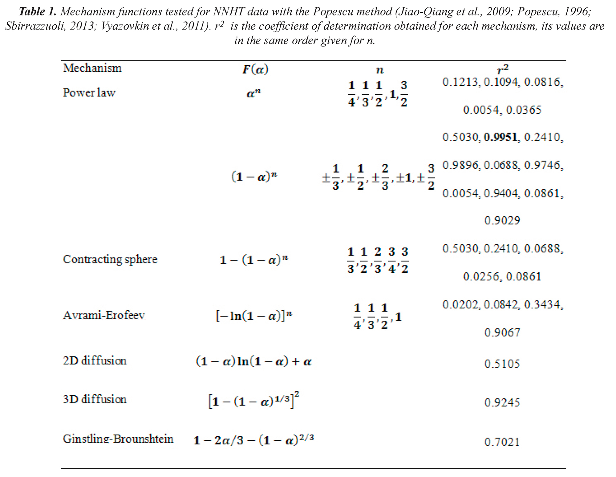
Figure 1. Experimental data for the the non-isothermal decomposition of 2-nitroimino-5-nitro-hexahydro-1,3,5- triazine (NNHT). Lines, from left to right correspond to heating rates β = 2, 5, 10, and 15K/min.

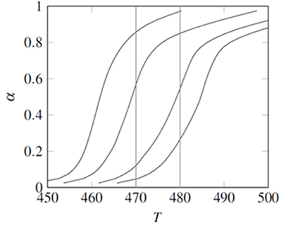
Figure 2. Isoconversional data fit example (activation energy for NNHT non-isothermal decomposition, (Jiao-Qiang et al., 2009) Results obtained with integration are represented with ○ (from Sr minimization), and + (from Φ minimization). Values obtained with integration are represented with Δ (from Sr minimization), and × (from Φ minimization).

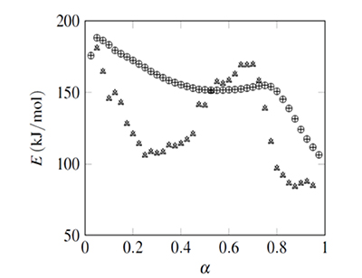
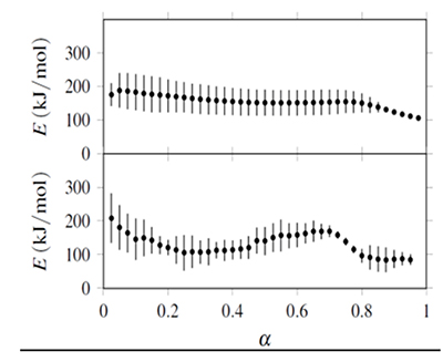
Figure 3. Confidence intervals (bars) for activation energies obtained from isoconversional analysis. Upper half: E obtained with ^... integration. Lower half: E obtained with integration.

The temperature integral was calculated with the incomplete gamma function, p(x)=Γ(-1,x) with T₀≈300K, estimated from the DSC curve shown in the data source (Jiao-Qiang et al., 2009). Using x₀=E⁄(RT₀) it was found that calculations made with and without p(x₀) terms produce the same result because p(x₀) values were very small. This suggest that the usual omission of p(x₀) does not influence parameter estimation.

The isoconversional analysis was applied to T sets corresponding to the four heating rates for each α, therefore the results are presented in Figs. 2 and 3 as functions of α in both variants, (Eqs. 15 and 16). The function Sr depends on two variables (E, ln A), and it was minimized using the Nelder-Mead algorithm, as included in the software Scilab. The initial estimates of E, ln A were 100 kJ/mol and 20 (similar to the results in the source of experimental data), and for each following α the minimization was started with the results from the previous extent of conversion.

The minimum of the function Φ(E) was found at each β value using the golden ratio method (Cai et al., 2010). A set of energy activation values was created calculating two E values with x=1 and x=100 for each T(β) measurement. Then, the biggest and smallest values of this set were used to start the search for the minimum with the golden ratio method. This procedure was repeated for each set of measurements to get E(α).

The confidence intervals were calculated at a 95% level from the joint parameter likelihood region associated to non-linear regression using Fisher's F distribution. This region is defined from

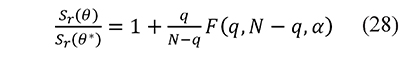
where θ* represents the parameter set (E, lnA) that minimizes S_r (Buzzi-Ferraris & Manenti, 2010; Mendenhall & Sincich, 2011). The value F is computed to an α confidence level with q parameters and N - q degrees of freedom associated to N observations. Equation 28 is solved for each parameter, and its respective confidence interval is the difference between the values of the parameter obtained with θ and θ*.

The activation energies, E, and their confidence intervals (error bars) are shown in Figs. 2 and 3. It includes values calculated with the four possible combinations, integration from α=0 or between consecutive αs, with minimization of Sr or Φ. The values of E obtained from the functions S_r and Φ were equal, and values from integration coincide with the E(α) curve obtained with Ozawa's method shown in the NNHT thermal decomposition paper (Jiao-Qiang et al., 2009). The integration implies a constant E value from the initial temperature to Tα producing values that vary smoothly, with confidence intervals that tended to reduce with α. On the other hand results from integration, and their associated confidence intervals, showed no clear tendency.

4. Conclusions

The temperature integral can be evaluated univocally with the incomplete gamma function, even in cases where the preexponential factor depends on the temperature. The use of the function Γ instead of an approximation to p(x) allows reducing isoconversional and non-isoconversional integral analysis of data to a non-linear regression of parameters. Nevertheless, there remains a poignant question: is the use of Γ an approximation by itself? In brief the answer is "no", but we will extend such answer drawing an analogy between the functions Γ(a,x) and exp(x). Results of e^x from calculators or numerical software are not considered approximations because they are the best possible values within system's floating point arithmetic. In the same way Γ is calculated in the most accurate possible way using continued fractions until the addition of more terms does not produce more digits, as described in the supplementary material.

Availability of non-linear regression methods in current numerical software makes them as easy to apply as linear regression to find the values of A and E, but the researcher should be aware that it results necessary to cast the minimization function in terms of x=E⁄RT and lnA in order to avoid numerical conditioning problems related with the use of terms with very different orders of magnitude. It is also true that the proposed unified procedure, being based on a non-linear regression, requires initial estimates of E and ln A, but they can be obtained from some other method based on linear regression, or chosen from previous results for similar samples. Another possible objection is that different minimization methods could give different parameters for the same data set, replicating the problem posed by the use of approximations. But given that the objective function is the same, and supposing that the methods are equally capable they should locate the same minimum. There remain, however, the effects of starting from different initial estimates, the hypothetical presence of local minima, or limitations in the algorithms. An extensive analysis of all these factors is beyond the scope of this paper; although it could be addressed in future work. In the same way this unified interpretation can be applied to the discovery of more complex reaction mechanisms and kinetics.

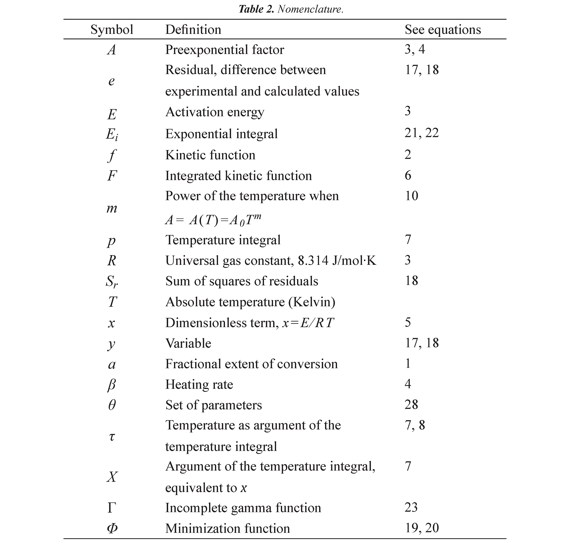
Table 2. Nomenclature.

5. References

Aranzazu-Ríos, L.M., Cárdenas-Muñoz, P.V., Cárdenas-Giraldo, J.M., Gaviria, G.H., Rojas-González, A.F. & Carrero-Mantilla, J. I. (2013). Modelos cinéticos de degradación térmica de polímeros: una revisión. Revista Ingenierías Universidad de Medellín, 12 (23), 113-130.         [ Links ]

Arrhenius, S. (1889). Uber die reaktiongeschwindigkeit bei der inversion von rohzucker durch sauren (On the reaction velocity of the inversion of cane sugar by acids). Zeitschriftfur physikalische Chemie, 4 (1), 226-248.         [ Links ]

Askey, R.A. & Roy, R. (2010). Gamma Function. In, F. W. J. Olver, D. W.Lozier, R. F. Boisvert & C. W. Clark (Eds.) NIST Handbook of Mathematical Functions (Chapter 5). Cambridge, UK: Cambridge University Press.         [ Links ]

Blaine, R., & Kissinger, H. (2012). Homer Kissinger and the Kissinger equation. Thermochimica Acta, 540 (1), 1-6.         [ Links ]

Brown, M.E., Maciejewski, M., Vyazovkin, S., Nomen, R., Sempere, Burnham, J.A., Opfermann, J., et. al. (2000). Computational aspects of kinetic analysis. Part A: The ICTAC kinetics project-data, methods and results. Thermochimica Acta, 355 (1), 125-143.         [ Links ]

Budrugeac, P. (2010). An iterative model-free method to determine the activation energy of non-isothermal heterogeneous processes. Thermochimica Acta, 511 (1), 8-16.         [ Links ]

Budrugeac, P. (2011). An iterative model-free method to determine the activation energy of heterogeneous processes under arbitrary temperature programs. Thermochimica Acta, 523 (1), 84-89.         [ Links ]

Buzzi-Ferraris, G., & Manenti, F. (2010). Interpolation and regression models for the chemical engineer: solving numerical problems. Weinheim, UK: Wiley-VCH.         [ Links ]

Burnham, A. K. (2000). Computational aspects of kinetic analysis. Part D: The ICTAC kinetics project - multi-thermal-history model-fitting methods and their relation to isoconversional methods. Thermochimica Acta, 355 (1), 165-170.         [ Links ]

Cai, J. & Chen, Y. (2012). Iterative linear integral isoconversional method: Theory and application. Bioresource Technology, 103 (1), 309-312.         [ Links ]

Cai, J., Han, D., Chen, C., & Chen, S. (2010). Application of the golden section search algorithm in the nonlinear isoconversional calculations to the determination of the activation energy from nonisothermal kinetic conversion data. Solid State Sciences, 12 (5), 829-833.         [ Links ]

Criado, J.M., Pérez-Maqueda, L.A., & Sánchez-Jiménez, P.E. (2005). Dependence of the preexponential factor on temperature. Journal of Thermal Analysis and Calorimetry, 82 (3), 671-675.         [ Links ]

Farjas, J. & Roura, P. (2011).Isoconversional analysis of solid state transformations: A critical review. Part I. Single step transformations with constant activation energy. Journal of Thermal Analysis and Calorimetry, 105 (3), 757-766.         [ Links ]

Flynn, J. H. (1997). The 'Temperature Integral' -Its use and abuse. Thermochimica Acta, 300 (1), 83-92.         [ Links ]

Flynn, J.H. & Wall, L.A. (1966). General Treatment of the thermogravimetry of polymers. Journal of Research of the National Bureau of Standards -A. Physics And Chemistry, 70A (6), 487-523.         [ Links ]

Jiang, Y., Liu, F. & Song, S. (2011). Improved analytical description for non-isothermal solid-state transformation. Thermochimica Acta, 515 (1), 51-57.         [ Links ]

Jiao-Qiang, Z., Hong-Xu, G., Li-Hong, S., Rong-Zu, H., Feng-Qi, Z., & Bo-Zhou, W. (2009). Non-isothermal thermal decomposition reaction kinetics of 2-nitroimino-5-nitrohexahydro-1,3,5-triazine (NNHT). Journal of Hazardous Materials, 167 (1), 205-208.         [ Links ]

Lyon, R. & Safronava, N. (2013). A comparison of direct methods to determine n-th order kinetic parameters of solid thermal decomposition for use in fire models. Journal of Thermal Analysis and Calorimetry, 114 (1), 213-227.         [ Links ]

Maciejewski, M. (2000). Computational aspects of kinetic analysis. Part B: The ICTAC kinetics project - the decomposition kinetics of calcium carbonate revisited, or some tips on survival in the kinetic minefield. Thermochimica Acta, 355 (1), 145-154.         [ Links ]

Mendenhall, W., & Sincich, T. A. (2011). Second Course in Statistics: Regression Analysis (7th ed.) New Jersey, USA: Pearson.         [ Links ]

Popescu, C. (1996). Integral method to analyze the kinetics of heterogeneous reactions under non-isothermal conditions a variant on the Ozawa-Flynn-Wall method. Thermochimica Acta, 285 (2), 309-323.         [ Links ]

Roduit, B. (2000). Computational aspects of kinetic analysis. Part E: The ICTAC kinetics project-numerical techniques and kinetics of solid state processes. Thermochimica Acta, 355 (1), 171-180.         [ Links ]

Sbirrazzuoli, N. (2013). Determination of pre-exponential factors and of the mathematical functions f(a) or F(a) that describe the reaction mechanism in a model-free way. Thermochimica Acta, 564 (1), 59-69.         [ Links ]

Vyazovkin, S. (1997) Evaluation of activation energy of thermally stimulated solid-state reactions under arbitrary variation of temperature. Journal of Computational Chemistry, 18 (3), 393-402.         [ Links ]

Vyazovkin, S., Wight, C. A. (1997). Kinetics in solids. Annual Review of Physical Chemistry, 48 (1), 125-149.         [ Links ]

Vyazovkin, S. (2000). Computational aspects of kinetic analysis. Part C. the ICTAC kinetics project - the light at the end of the tunnel? Thermochimica Acta, 355 (1), 155-163.         [ Links ]

Vyazovkin, S. (2001). Modification of the integral isoconversional method to account for variation in the activation energy. Journal of Computational Chemistry, 22 (2), 178-183.         [ Links ]

Vyazovkin, S., Burnham, A. K., Criado, J. M., Perez-Maqueda, L. A., Popescu, C. & Sbirrazzuoli, N. (2011). ICTAC kinetics committee recommendations for performing kinetic computations on thermal analysis data. Thermochimica Acta, 520 (1), 1-19.         [ Links ]

Wang, C. H. & Hsu, C. H. (2012). New nonisothermal Arrhenius temperature integral approximate formula. Environmental Engineering Science, 29, 964-971.         [ Links ]

Yunqing, H. (2014). Theoretical study of thermal analysis kinetics. Ph. D. Thesis, University of Kentucky. Lexington, USA.         [ Links ]

Revista Ingeniería y Competitividad por Universidad del Valle se encuentra bajo una licencia Creative Commons Reconocimiento