


 Inglés (pdf)
 Articulo en XML
 Referencias del artículo
 Enviar articulo por email
 Citado por SciELO
  Citado por Google
  Similares en
SciELO
Similares en
SciELO  Similares en Google
 Permalink
1. Introduction
Remote homology detection is a key problem Bioinformatics. Two proteins are remote homologs when they are structurally and functionally related but at the same time they keep a low sequence identity. The term remote homologs is related to proteins that share a common ancestor that is distantly related in an evolutionary way. Two remote homologs inherit their functions from a common ancestor. However, because of the mutations that occur in every protein, the primary sequences of two remote homologs are no longer similar to the amino acid sequence of the ancestor. Formally, two proteins are remote homologs if they have the same function and a sequence identity lower than the 25% 1. The main difficulty when detecting remote homologs is the fact that even though two remote homologs have the same function, there is no evidence in their primary sequences that reflects the evolutionary relationship.
The remote homology detection problem can also be understood by using the SCOP hierarchy (Structural Classification Of Proteins). In the SCOP database a four level hierarchy formed by family, superfamily, fold, and class levels, is used. Each level in the SCOP hierarchy has its own conditions. For instance, proteins with a high sequence identity that also have the same function are placed in the same SCOP family. Proteins with the same function are placed in the same superfamily without considering the sequence identity. Two remote homologs are proteins that belong to the same superfamily but at the same time they belong to different families, which means they have the same function but also a low sequence identity. Families and superfamilies have been used in the remote homology detection problem because we can easily identify proteins with the same function whose primary sequences no longer reflect an evolutionary relationship.
Three different approaches have been used when detecting remote homologs: pairwise sequence comparison, generative strategies, and discriminative methods. Currently, the discriminative methods are the only strategy that is being used to detect remote homologs. Discriminative methods are based on the idea of having positive and negative datasets and building a classifier that is able to detect remote homologs. Discriminative methods are divided in more specific categories: sequence composition-based methods and profiled-based methods. Sequence composition-based methods use a transformation step in which a vector of values is obtained from an amino acid sequence. The transformation can occur by counting some specific amino acids or physicochemical properties. For instance, in the SVM-PCD method 2, amino acid sequences are transformed by using 531 physicochemical properties which are available in the AAindex 3. The SVM-PCD method takes an amino acid sequence and transforms it by using each physicochemical property separately. Then, the addition of the transformed values of every four consecutive amino acids is calculated. A sliding window of size four is shifted over the sequence obtaining the sum of every four values. Then, a distribution of the sums is obtained by using 18 frequency values. A distribution allows to determine which ranges of values are more frequent than others. This process is repeated 531 times, one time for each physicochemical property and a total of 18*531=9558 values are obtained. Another sequence composition-based method is SVM-RQA 1. In the remote SVM-RQA method a total of 480 physicochemical properties are used. For each property, the amino acid sequence is transformed and then a recurrent quantification analysis is applied on the transformed sequence 4. The recurrent analysis allows to obtain 10 values that capture the most relevant information about the transformed sequence. The SVM-RQA method uses a total of 480*10=4800 values to represent a protein. In the SVM-PDT method 5 531 physicochemical properties are used. For each transformed sequence the distances between every pair of amino acids that are separated by λ residues are calculated. For instance, the distances between every two residues are calculated when λ=2. Then, the average distance is calculated. In the SVM-PDT method λ is used from 1 to 8. Therefore, a total of 531*8=4248 values are used to represent a protein. The difference between the sequence composition-based methods relies on the calculation that is performed over the transformed sequence. The calculation tries to capture the most relevant information about the protein. The ROC score (Receiver Operating Characteristic) of the sequence composition-based methods ranges from 0.89 y 0.92.
Profile-based methods use evolutionary information that is obtained from a multiple sequence alignment against a non-redundant database. A profile allows to identify which amino acids are evolutionary related. Because there is an evolutionary relationship between two remote homologs, the profiles have shown to be useful when detecting remote homologs. The ROC score of the profile-based methods is 0.95.
In this paper, we propose a new remote homology detection method called remote-3DD, which uses physicochemical properties of the amino acids and predicted contact maps. Predicted contact maps are a 3D representation of the protein that can be obtained from the amino acid sequence. The rest of the article is organized in sections. Section 2 explains every step of the remote-3DD method. Results are presented and discussed in Section 3. Finally, the conclusions are shown in Section 4.
2. Methodology
The remote-3DD method uses both contact maps and distributions of the interaction matrix. This method is proposed as a strategy for improving the accuracy (i.e., ROC score) of the remote-C3D method 6, which uses contact maps alone. We hypothesize that the accuracy of the remote-C3D method can be improved by incorporating the distributions of the interaction matrices. The remote-3DD method is formed by the following four steps: (1) Obtaining the models using physicochemical properties and actual contact maps, (2) Predicting contact maps and calculating interaction matrices, (3) Calculating the count vectors, (4) Obtaining a classifier for each family in the dataset. Every step is explained in detail as follows.
2.1. Obtaining the models
A protein can be represented as a contact map, which is obtained by discretizing its corresponding distance matrix. A distance matrix holds the Euclidean distances between every pair of residues. The distances are calculated in Angstroms, which are 1x10⁻¹⁰ meters. When the distance between two amino acids is less than or equals to 8 Angstroms they are considered to be close, and otherwise, they are far from each other. A contact map collects the information about the amino acids that are close (i.e., contacts) and those that are far from each other (i.e., non-contacts). The importance about obtaining the contact map of a protein is that it represents the 3D shape of the protein. Figure 1 shows on the left the contact map for protein d1ceqa1, whose SCOP code is.2.1.5. Contacts are represented in black and non-contacts in gray. According to Choi et al. 7, even though proteins can have different 3D shapes, and thus, different contact maps, there are common submatrices of the distance matrices that can be found in different proteins. These common submatrices are used as models in some remote homology detection methods 6,7. The models in the remote-3DD method are submatrices of the contact maps and distributions of the interaction matrices that commonly occur in different proteins. An interaction matrix holds the additions of the physicochemical values of every pair of amino acids. Figure 1 shows on the right the interaction matrix when the physicochemical property “Hydropathy index” is used.
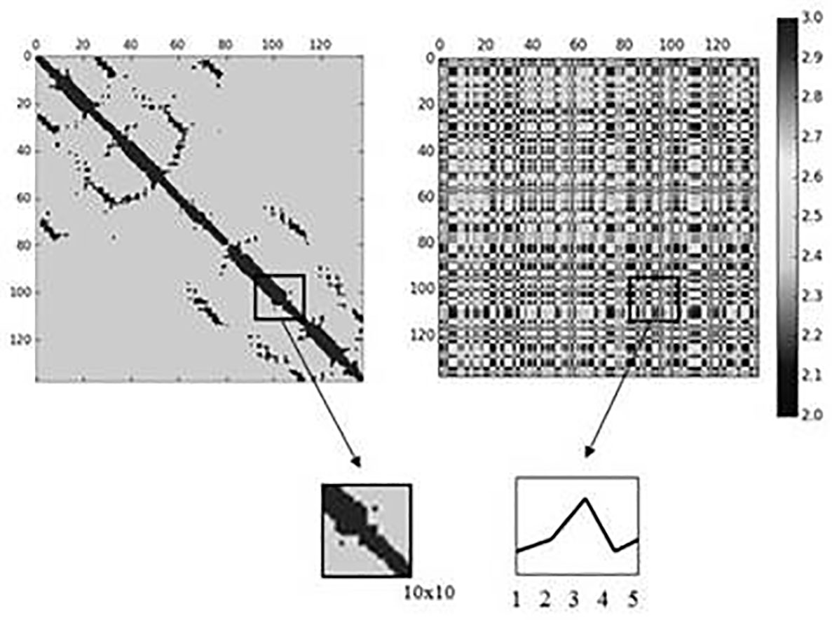
A specific dataset formed by proteins represented as contact maps and interaction matrices are used to obtain the models. In this research we use the same methodology presented in Choi et al. 7 to obtain the models. However, in the remote-3DD method both contact maps and distributions of the interaction matrices are used. A structural fragment is obtained by using submatrices of size mxm from both the contact map and the interaction matrix. Then, a five bin distribution of the values in the submatrices of the interaction matrix is obtained. Every structural fragment is formed by m*m+5 values, where mxm values are obtained from the contact map and five values from the distribution. The values in the interaction matrix are in the interval 2,3. A distribution of every mxm submatrix in the interaction matrix is calculated by using the intervals (2.0-2.2), (2.2-2.4), (2.4-2.6), (2.6-2.8), and (2.8-3.0). A distribution holds the frequency in which each interval occurs in a given submatrix. Figure 1 shows the process of obtaining the structural fragments when 10x10 submatrices are used. In this case, each structural fragment has 105 values; 100 values obtained from the submatrix of the contact map and five values from the distribution of values in the submatrix of the interaction matrix.
The models in the remote-3DD method are obtained by using a clustering algorithm named CLARA 8. We use a clustering algorithm because it allows dividing a dataset into groups whose objects are similar to each other. When a clustering algorithm is used, a set of medoids are obtained. Each group has a corresponding medoid that represents the typical values that are part of the cluster. The medoids obtained by the clustering process are used as models in the remote-3DD method.
Obtaining the models starts by calculating the structural fragments of m*m+5 values from a specific dataset. Each structural fragment in the remote-3DD method is formed by a submatrix of the contact map and a distribution of the values in the corresponding interaction submatrix. The CLARA algorithm is used on every protein to obtain a total of 50 medoids, which are the most representative structural fragments. Then, the 50 medoids of all proteins that are part of the specific dataset are clustered again using different number of clusters (i.e., k=10, 20, 30, 40, y 50). This number of models are used when testing the method and are discussed in section 3. The clustering process is divided in two steps because we obtained thousands of submatrices from the specific dataset, which affects the performance of the clustering algorithm. For instance, when we use a protein with 150 amino acids and 10x10 submatrices, a total of (150-10+1)*(150-10+1)=19881 submatrices are obtained. As observed, the performance of the clustering process would be affected with the number of submatrices considered in this research.
2.2. Predicting contact maps and calculating interaction matrices
The second step in the remote-3DD method is about predicting the contact maps and calculating the distributions of the interaction matrices for all proteins in the dataset. The remote homology detection problem occurs when the 3D shape of the protein is still unknown and only the amino acid sequence is available. Being able to predict the function of a protein whose 3D shape is still unknown becomes the main reason why we want to predict remote homologs. Detecting remote homologs allows identifying the proteins that are functionally related. Unlike the process of obtaining the models, which is performed by using actual contact maps, the second step of the remote-3DD method predicts the contact maps of every protein in the dataset by using the amino acids sequences. In addition, the distribution of the interaction matrix is also calculated.
In this research, the NNcon1.0 program 9 is used to predict contact maps. NNcon1.0 uses neural networks to predict whether two residues are in contact. In addition, another neural network is used to detect anti-parallel beta-sheets, a 3D conformation that is difficult to predict. The predicted contact map for a protein with n residues is represented as a nxn matrix where each position (i,j) indicates whether the residues i and j are in contact. The values 1 and 2 are used to indicate contacts and non-contacts, respectively.
The interaction matrix is calculated by using a given physicochemical property. The AAindex has 544 physicochemical properties available. Each physicochemical property is represented as a table that indicates the specific value of the corresponding property for the 20 amino acids. For instance, by using the “Hydropathy index” we are able to know that the hydropathy values of the Alanine, Asparagine, and Cysteine, are 1.8, -3.5, and 2.5, respectively. Each physicochemical property has a different range of values, and thus, the first step when obtaining the interaction matrix is about scaling the values to the range 2,3. This specific range is chosen trying to make the values in the interaction matrix and the contact maps comparables. Finally, for each pair of amino acids i and j, the addition between the scaled values is calculated. For an amino acid sequence of n residues, a nxn matrix representing the interactions between every pair of amino acids is obtained.
2.3. Calculating the count vectors
A count vector holds the number of times that each model is observed in the predicted contact map and in the interaction matrix of a given protein. Representing a protein as a count vector allows comparing whether two proteins use the same models. Models are associated with common 3D shapes, and thus, it is expected that two proteins with similar 3D shapes have similar counts of the models. The models obtained in section 2.2. are used to obtain the count vectors. First, the structural fragments are extracted. Each structural fragment is obtained from the submatrices of the contact map and the interaction matrix. The remote-3DD method takes each structural fragment and calculates the Euclidean distance to the k models. A structural fragment is assigned to the model whose distance is the lowest. When each submatrix in a given protein P is assigned, it can be represented as the number of times that each model is observed. The count vector holds those values. A characteristic model is the empty model, which represents a submatrix that has no contacts. The empty model is the most frequent model in any protein. Because of the difference between the number of times that the empty model is observed in any protein compared to the rest of the models, a normalization process has to be done.
The normalization process performed in the remote-3DD method is the same used in the LFF method 7. A count vector for a protein P is defined as VCP=[f(P,1),f(P,2),…,f(P,k)], where f(P,i) is the number of times that the model i occur in a protein P. The normalized count vector for a protein P is calculated as VCNP=[AP1,AP2,…,APk], where APi is defined in Eq. 1
 (1)
(1)
where f(P,i) is the value in VCp and indicates the count for the i-th model of a protein P. In addition, D is the dataset that is used during the normalization process.
2.4 Building a classifier for each family in the dataset
Discriminative methods are based on obtaining a classifier that is able to detect remote homologs. Most of the current methods use Support vector machines (SVM) as the classification technique. A classifier in the remote homology detection problem allows predicting whether a given protein is a remote homolog of a specific family. Two class labels are used in the classifier when detecting remote homologs, +1 and -1, where +1 represents that a given protein is a remote homolog, and -1, otherwise. SVMs are the most popular technique because they can handle high dimensionality in the dataset. Every protein is represented by thousands of values when detecting its remote homologs. For instance, the SVM-PCD and SVM-PDT methods use 9558 and 4248 values, respectively. However, in the remote-3DD method we use count vectors with low dimensionality (i.e., at most 50 values). Because of the low dimensionality we are able to consider some classifications techniques that have not been used in this specific problem. The resulting classifiers obtained in the remote-3DD method can be used by biologists to detect remote homologs. These classifiers allows identifying which families are functionally related to a given protein and at the same keeping a low sequence identity.
Seven classification techniques are used in the remote-3DD method. The selected strategies have been used in previous works in Bioinformatics. In this research, we use a subset of the strategies used by Kukreja et al. 10 in which 18 algorithms were used on datasets related to Diabetes type I, Alzheimer and antibodies. The selected classification algorithms are: NaiveBayes, BayesNet, BayesMultinomial, Multilayer perceptron, HyperPipes, LMT (logistic model trees) and VFI (voting feature intervals). A classification technique is selected for each SCOP family in the dataset. The training dataset for each SCOP family is divided into two parts, t1 and t2. We use the first part (t1) to train the classification models considering the seven classification techniques separately, which means that seven classifiers are obtained. Then, the classifiers are tested using the part t2. This process is executed again exchanging t1 and t2 by using t2 for training and t1 for testing. A total of 14 classifiers are obtained from the training dataset. Then, the classification technique with the highest ROC score is selected as the classification strategy of a given family. Finally, the selected strategy is used with the whole training dataset and it is tested with the test dataset. The results are shown in section 3.
3. Results and discussion
Two different SCOP versions were used during testings, the SCOP 1.53 and SCOP 1.55 datasets. Theses datasets are filtered using the same strategy proposed by Liao & Noble 11. For each family f, proteins inside f are considered the positive test set and proteins outside f but in the same superfamily are taken as the positive training set. In addition, proteins outside the fold where f belongs to are considered the negative dataset. When detecting remote homologs only families with at least 10 proteins in the positive training set and five proteins in the positive test set are used. Therefore, after filtering the SCOP 1.53 dataset a total of 54 families are obtained. The 54 families that are used when detecting remote homologs in the SCOP 1.53 dataset is presented by Liao & Noble 11. The SCOP 1.55 dataset has 3527 proteins and 51 families after the filtering process. The 51 families that are used when detecting remote homologs in the SCOP 1.55 dataset is presented by Bedoya & Tischer 6. Tests also include different size of submatrices (4x4, 6x6, 8x8, 10x10 y 12x12), number of models (10, 20, 30, 40, y 50), and three physicochemical properties (Alpha helix propension, Hydropathy index, and pK (-COOH) index). These physicochemical properties were selected because they have shown excellent results in previous works 1,2.
A key aspect in the remote-3DD method is the specific dataset that is used to obtain the models. A clustering algorithm is applied on a specific dataset and the resulting medoids are used as models. In this research, a total of 40 proteins were used in the specific dataset that is used to obtain the models. Considering that the SCOP 1.55 dataset has 3527 proteins, 51 families and 20 superfamilies, two proteins for each superfamily were selected. It is expected that this specific dataset represents the diversity in the whole dataset, and thus, the clustering process can detect the most common submatrices and distributions. It is also expected that each superfamily has some submatrices of the contact maps and some distributions that are specific and different from the rest of the superfamilies.
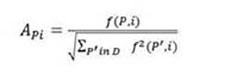
Figure 2 shows the models that are obtained when 10x10 submatrices and the physicochemical property “Hydropathy index” are used. Figure 2(a) shows the part of the models that are obtained by using the contact maps and Figure 2(b) show the distributions for each model. The x-axis in Figure 2(b) represents the intervals of the distributions. The intervals (2.0-2.2), (2.2-2.4), (2.4-2.6), (2.6-2.8), and (2.8-3.0), are represented by integer numbers 1, 2, 3, 4 and 5, respectively. In the y-axis the frequencies of each interval are shown. For instance, model m2 has the frequencies 0.00, 0.04, 0.43, 0.42, 0.11, for the five intervals. As can be observed, each model is represented by two parts, which are the 3D information and the distribution of values. The 3D information of a model reflects the common 3D conformations. For instance, model m1 is a conformation that can be found in an alpha-helix and model m6 can be observed in a beta-sheet. In addition, model m9 is a submatrix that is usually observed in an anti-parallel beta-sheet. Models reflect the most common 3D conformations that can be observed in proteins.
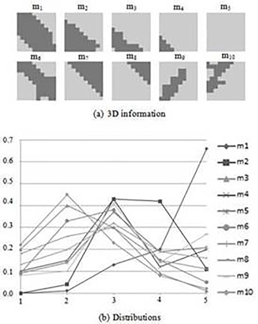
Figure 2 Models used in the remote-3DD method when 10x10 submatrices and the physicochemical property “Hydropathy index”are used.
3.1. Evaluation on the SCOP 1.53 dataset
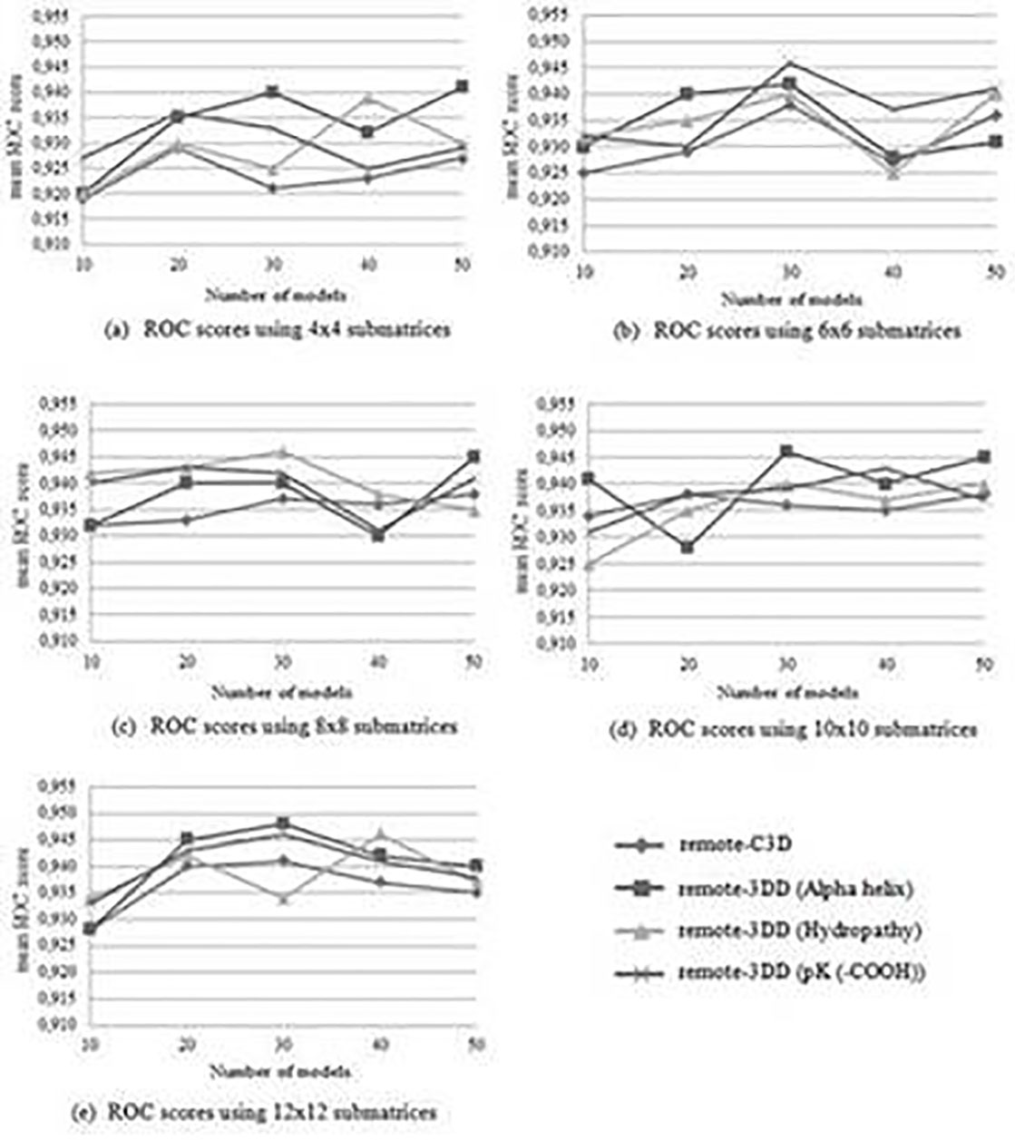
Figure 3 shows the results when testing the remote-3DD method using different sizes of submatrices and number of models. In addition, the accuracy (i.e., ROC score) of the remote-C3D method is also shown. As observed, the remote-3DD method outperforms the remote-C3D method in most of the experiments. For instance, Figure 3(e) shows the accuracy values when 12x12 submatrices are used. It can be observed that is better to use the models that include physicochemical properties rather than using the 3D information alone as in the remote-C3D method. Three out of two physicochemical properties reach a higher accuracy than using the remote-C3D method when 4x4 are considered. The highest improvement during testings is obtained when 12x12 submatrices, 50 models, and the “Alpha helix propensity”, are used. In this case, the ROC score goes from 0.912 in the remote-C3D method to 0.940 in the remote-3DD method. Other high improvements are: 0.023, reached when using 12x12 submatrices, 50 models and the “Hydropathy index”; and 0.021, with 12x12 submatrices, 40 models, and the “Alpha helix propensity”. Another size of submatrix that showed significant improvements is 10x10. For instance, accuracy values of 0.018 when 30 models and the “Hydropathy index” are used, and 0.017 when 30 models and the “Alpha helix propensity” are selected. The highest ROC score reached by the remote-3DD method is 0.954 and the lowest ROC score is 0.920. The results obtained during testings indicate that including physicochemical properties in the representation of the structural fragment improves the accuracy of the remote homology detection. According to Yang et al. 1, the relationship between two proteins that are distantly related can be observed in their physicochemical values even though their amino acids sequences no longer show any kind of similarity.
3.2. Evaluation on the SCOP 1.55 dataset
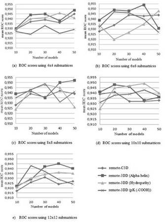
Figure 4 shows the mean ROC score and the standard deviation for the 51 families in the SCOP 1.55 dataset when both the remote-C3D and the remote-3DD are used. In this case, submatrices of 4x4 reached a higher accuracy than the remote-C3D method for all number of models, size of submatrices, and three physicochemical properties. The results indicate that in the SCOP 1.55 dataset is better to use 3D information along with physicochemical properties rather than using 3D information alone. The highest improvement is 0.028, which is reached when 4x4 submatrices, 30 models, and the “Alpha helix propensity” are used. In this case, the ROC score goes from 0.921 in the remote-C3D method to 0.949 in the remote-3DD method. In addition, when the physicochemical properties “Alpha helix propensity”, “Hydropathy index”, and “pK (-COOH) index” are used, there are improvements in the ROC scores that go from 0.920 to 0.948, 0.919 to 0.946, and 0.927 to 0.946, respectively.
3.3. Comparison with the existing methods
Sequence composition-based methods reach a ROC score of 0.92. For instance, the accuracy of the SVM-RQA, SVM-PDT, and SVM-PCD methods, are 0.912, 0.916, and 0.906, respectively. Profile-based methods reach ROC scores of 0.950. For instance, the accuracy of the SVM-PDT-Profile and SVM-DT methods are 0.950 and 0.948, respectively. The ROC scores of the SVM-RQA, SVM-PDT, SVM-PCD, SVM-PDT-Profile and SVM-DT methods, were all obtained by using the SCOP 1.53 dataset, which is the same dataset used in this research. The ROC score of the remote-3DD method ranges from 0.920 to 0.954 when the SCOP 1.53 dataset is used. According to the results, the remote-3DD method reach higher ROC scores than the sequence composition-based methods and in some cases comparable accuracy values to the profile-based methods. In addition, the results also allowed to prove the hypothesis in this research, which is about improving the accuracy of the remote-C3D method. The improvement is due to the fact that the remote-3DD method uses models that have more information than the remote-C3D method. It allows each model to be more different from the rest of the models than they are in the remote-C3D method, which helps the assignation process when the models are used to represent a protein.
4. Conclusions
In this paper, a new remote homology detection method was presented. The proposed method uses both predicted 3D information and physicochemical properties. Unlike the current methods, the remote-3DD method uses distributions of the values in submatrices taken from the interaction matrix. The ROC scores obtained when testing the remote-3DD method showed that the proposed method reach higher accuracy values than the sequence composition-based methods and, in some cases, depending on the physicochemical property, the number of models, and the size of submatrices, a comparable accuracy to the profile-based methods. In addition, the hypothesis established for this research was proved, which means that we were able to improve the accuracy of the remote-C3D method by using physicochemical properties. The improvement in the ROC score is due to the fact that the physicochemical properties are conserved between two remote homologs. The remote-3DD method can be used by biologists who have a given protein represented as an amino acids sequence and whose function is still unknown. Detecting remote homologs allows identifying the superfamilies and families related to a given protein, which helps to understand what proteins are functionally related. We propose to include more physicochemical properties in the experiments, and also to achieve a strategy that allows us to use different physicochemical properties at the same time and not separately as it was done in this research.

