


 English (pdf)
 Article in xml format
 Article references
 Send this article by e-mail
 Cited by SciELO
  Cited by Google
  Similars in
SciELO
Similars in
SciELO  Similars in Google
 Permalink
1. Introduction
Natural hydraulic behaviour is very complex, which is why theoretical simplifications that facilitate the analysis of natural channels are made in hydraulics 2. However, these simplifications eliminate characteristic that manifest themselves in real flows, such as viscosity, rotationality and compressibility. This generates uncertainty in the results, which increases when working with bi-phased flows. Taking the number of solids in a flow into account, its rheology can change drastically, changing from a Newtonian to a non-Newtonian fluid 3,4.
The problem that is approach in this investigation is related to the effects that might occur on the surface levels of water in the curving of a canal when solid particles are added in different concentrations.
Hydraulic phenomena can be analysed using analytic, numerical, and experimental models. Analytic models make approximations to the behaviour of the fluid using empirical simplifications and applicable equations for fluids without solids 5. Numerical simulation models 6,7 solve complex equation systems for the processing of data 8,9, allowing for approximations that are closer to reality. Experimental models 5,10,11, are generally smaller scale reproductions that are used to delimitate variables that intervene in a phenomenon, and can be used to obtain statistics or empirical equations that explain it 10,12.
The previously presented methods will be used in this study to analyse the effects produced by the concentration of solids in the behaviour of the phenomenon of superelevation 11,13,14. This hydraulic phenomenon presents itself in open canals with curved alignments and is characterized by an increase in the height of the flow at the external wall of the curve and a decrease at the inner curve 2. Usually, in engineering, this phenomenon is approached through equations that do not take the solid phase of the flow into account 2,15. The purpose of this study is to make a contribution towards the understanding of this phenomenon, which can occur in mudflows, inundations or river floods. All of these events can pose a great threat to infrastructure and to life.
Mudflows or lahars 3,16,17, are flows with a high concentration of solids, which can range from 20% to more than 60% of the total volume of the flow 4,18-20. These flows do not behave as Newtonian fluids since the shear stress and the velocity gradient do not have a linear relationship. 4,21.
The purpose of this work is to make a physical and numerical investigation using an experimental model, in order to make laboratory tests in an artificial canal, controlling the percentage of solids as well as the slope at the entrance of the curve. Additionally, the work intends to make numerical simulations, using the specialised software TITAN2F 9,22, in which the initial conditions used in the laboratory are replicated, thereby obtaining results about velocity and superelevation. Finally, the results obtained from both methods are compared to an analytical mathematical model that applies the second law of Newton, and a simplification of the velocity profile of the cross section of the canal 2.
2. Methodology
2.1. Experimental model
According to Baird 23 and Gutiérrez & Salazar 24, among others, an experimental design is defined as an application of the scientific method consolidated as a group of statistical and engineering techniques, that have been widely used in investigations with the purpose of understanding the functioning of a system or of a phenomenon.
With this in mind, a series of experiments were carried out, in which controlled changes were made in specific variables, such as the slope and the percentage of solids, in order to observe and understand the relationship between the cause and effects of these variables in the superelevation phenomenon.
A variety of studies have been made for the explaining and predicting of this phenomenon, such as 2,10,14,25, all of which have created good approximations of the event for pure fluids. These approximations generally only require geometrical and velocity parameters for their solutions, with the advantage that they only predict the maximal superelevation and it is not possible to know at what angle of the curvature it happens, like for example in equations 1, 2, and 3 2,26.
Where b is the width of the canal, Vz is the velocity at the entrance of the curve. g is gravity and 𝑟𝑐 is the radius of the curvature.
Where 𝑟0 is the external radius and 𝑟𝑖 is the internal radius.
Where 𝑉max is the maximum velocity of the cross sections before reaching the curve.
In these equations, ∆ℎ is the superelevation as the difference between the minimum and maximum level in a section of the curve. Out of these equation, the one that is used the most is equation 1, which can be deduced from a simple dimensional analysis.
2.1.1. Construction of the artificial canal
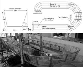
The canal was designed with a trapezoidal cross section measuring 0.3m and a height of 0.28m (Figure 1a) and is divided into three zones. The first zone is straight (Figure 1b). At its start, a compartment with a capacity of 50 litres was placed. This zone has a variable slope between 0% and 12.5%. The second zone is a 180° curve, as shown in (Figure 1b), with a varying bottom slope which varies along the way, which will be used in future studies. Finally, the last zone is a straight path with a constant slope at 2%, and ends in a curve that leads to a supplying tank.
2.1.2. Choice of variables
The parameters analysed in the phenomenon being studied are: the longitudinal slope, the concentration of solids, volume, and the shape of the canal. Since the laboratory assembly has specific dimensions (Figure 1), the variables to be controlled were reduced to the slope of the canal and the concentration of solids.
2 different slopes were considered, at 5% and 10%. Likewise, taking into account that the mixing system has a maximum limit of 30% solids, the range being evaluated will be from 0% to 30% solids in volumetric percentage. By using increases of 5%, this range was divided between 7 values: 0, 5, 10, 15, 20, 25, 30 percentage of solids. However, for the analysis of the information obtained, the number of solids deposited in the first section of the straight path is taken into account.
The tests were made at a room temperature of approximately 16° C. The solid phase was made out of sand with a mean diameter of 1 mm, and a density of 2.5 g/cm3. The fluid has a monodisperse, non-colloidal distribution.
With the purpose of analysing the results from equations 1, 2, and 3, experiments were made with pure water. From these experiments, the theoretical velocity using each of the equations was deduced. Tables 1 and 2.
Table 1 Results of theoretical velocities and experimental velocities with a 5% slope for pure water 5% superelevation of 0.176 m).
| Descripción | Velocidad | % Error | |
|---|---|---|---|
| Velocidad Experimental | 2.200 | m/s | ------------- |
| Ecuación 1 | 2.210 | m/s | 0.53 |
| Ecuación 2 | 2.200 | m/s | 0.06 |
| Ecuación 3 | 3.020 | m/s | 27.20 |
Table 2 Results of theoretical velocities and experimental velocity with a 10% slope for pure water (over- elevation of 0.218m).
| Descripción | Velocidad | % Error | |
|---|---|---|---|
| Velocidad Experimental | 2.543 | m/s | -------------- |
| Ecuación 1 | 2.463 | m/s | 3.31 |
| Ecuación 2 | 2.452 | m/s | 3.79 |
| Ecuación 3 | 3.365 | m/s | 24.38 |
Taking the results of Tables 1 and 2 into account, it was decided that equations 1 and 2 would be used, since they give results that are close to those observed in the laboratory.
2.1.3. Size of the sampling
With the intention of confirming that the sample size has statistical validity, it is necessary to obtain a sample that represents it. For this end, equation 4 was used, 27,28, in which 𝑛 is the size of the sample, 𝑘 is the corresponding value of the Gauss distribution 28, 𝑝 is the prevalence of the parameter to be evaluated, and e is the percentage of error that will be allowed. Finally, 𝑛 was calculated for different conditions of the level of confidence and percentage of error allowed, from which Table 3 was obtained.
Table 3 Number of tries depending on the level of confidence and the percentage of error allowed. (3 levels of confidence for each % of error).
| Nivel De Confianza | E | K | p | 1-p | n | Número Total de Ensayos |
|---|---|---|---|---|---|---|
| 95 | 0.05 | 1.96 | 0.5 | 0.5 | 384 | 5376 |
| 90 | 0.05 | 1.65 | 0.5 | 0.5 | 272 | 3808 |
| 85 | 0.05 | 1.44 | 0.5 | 0.5 | 207 | 2898 |
| 95 | 0.1 | 1.96 | 0.5 | 0.5 | 96 | 1344 |
| 90 | 0.1 | 1.65 | 0.5 | 0.5 | 68 | 952 |
| 85 | 0.1 | 1.44 | 0.5 | 0.5 | 52 | 728 |
| 95 | 0.15 | 1.96 | 0.5 | 0.5 | 43 | 602 |
| 90 | 0.15 | 1.65 | 0.5 | 0.5 | 30 | 420 |
| 85 | 0.15 | 1.44 | 0.5 | 0.5 | 23 | 322 |
With the data obtained from Table 3, and considering a level of confidence of 90% and a percentage of error of 15%, a sample of 30 tries for each scenario is obtained, for a total of 420 tries.
2.1.4. Experimental procedure
In order to carry out the experiments, two video cameras were placed over the canal. The first one was placed at zone one, recording facing its bottom, where position marks were placed every 10 cm, with the intent of determining the velocity that the flow passed with at that sector. The second one was placed at zone two, facing the scales that were placed at the outer wall of the canal, in order to register the maximum height that was produced by the superelevation phenomenon.
Then, the granular material was loaded inside the initial compartment and the rest of the control volume was filled with water. After this, the mixing device was activated and the flow was released. It is worth noting that the mixing was carried out with two rotors with 800 W of potency, and the homogeneity control proved difficult.
2.2. Digital modelling with Tita2F
TITAN2F is a software developed by PhD. Gustavo Córdoba at University of Buffalo, United States, for the numerical simulation of the behaviour of bi-phased flows over a digital terrain model 9. TITAN2F takes the dynamics of the solid material into account through the Mohr-Coulomb model and combines it with hydraulic models by using shallow waters equations. The interaction between the two phases is determined through a semi-empirical equation that relies on the percentage of solids 22.
The software requires the input of the initial conditions of the mud flow that is to be modelled, such as: volume, location, the digital terrain model over which the modelling will be carried out, the concentration of solids, the duration of the simulation, among other 9.
2.2.1. Construction of the digital model
The digital elevation model DEM, is a digital or computational representation usually of the geomorphology of a terrain. It is equally useful for representing the morphology of any element like streets, houses, cities and/or canals.
DEMs have been evolving in precision 29-31 as well as in their own generation method 32-34, in such a way that they allow for a great number of analysis with re-creatable, accessible, and trustworthy results 3,35.
DEMs are used in numerical modelling that is developed through software tools, as is the case of TITAN2F 9, LAHARZ 36,37, COMSOL Multiphysics, FLOW 3D 7,38, among others. It is worth noting that with a higher resolution comes a higher computational cost of the calculations that are made through it.
The DEM was built from the dimensions of the artificial canal (Figure 1), through a three-dimensional scheme made in AutoCAD Civil 3D™ (academic version), from which a vectoral representation of the canal was obtained with a precision of 0.01 m (Figure 2)
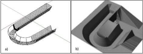
Figure 2 a) Scheme of the canal in AutoCAD Civil 3DTM(academic version). b) representation of the DEM in GRASS GIS.
Once the vectoral representation is obtained, it was imported to the Geographical Information System GRASS GIS, a free use software that is compatible with TITA2F 22. Once it has been imported, we use the command r.fillnulls 39 which is part of GRASS GIS, which completes the remainder of the information through interpolations in order to generate a single surface (Figure 2).
2.2.2. Entry data
The entry data used in order to execute the model are: the concentration of solids in a range between 5% and 30%, the location of the pile in the DEM file, the volume of the pile (40 litres) and a simulation time of 5 seconds.
When executing the TITAN2F program, a set of matrixes stored in plain text files (*.txt) was obtained. These were made out of 7 columns, which contain position at x, y, z, the thickness or height of the flow, the velocity, the concentration of solids and the dynamic pressure, respectively. Each matrix represents the flow in a specific timeframe.
3. Results
3.1. Experimental results
The obtained videos were processed for the obtainment of data, extracting time differences and distance travelled from the first camera, from which the entrance velocity at the curve was deduced. The height of the super elevation was observed directly from the second camera. Also, the quantity of material that deposited itself in zone one was weighed, in order to determine the percentage of solids that reached the curve. With these results, the density of the mix, according to equation (5), was calculated. The averages and statistical analysis obtained were registered in Table 4.
In this equation ⍴ 𝑚 is the density of the mix, ⍴𝑓 is the density of the fluid, ⍴ 𝑠 is the density of the solid and 𝜗𝑠 is the volumetric percentage of solids in the mix.
Table 4 Averages of the experimental results, percentage of solids, velocity and height of the superelevation.
| Canal Slope (%) | Percentage of Initial Solids (%) | Percentage of Solids at the Curve Entrance (%) | Mix Density ρ_m (Kg/m3) | Velocity at Curve Entrance (m/s) | superelevation ΔH (m) |
|---|---|---|---|---|---|
| 5 | 0 | 0 | 1000.00 | 2.204 | 0.176 |
| 5 | 3.4 | 1051.25 | 1.971 | 0.171 | |
| 10 | 6.9 | 1103.75 | 1.91 | 0.147 | |
| 15 | 10.4 | 1156.25 | 1.816 | 0.146 | |
| 20 | 13.9 | 1208.75 | 1.787 | 0.138 | |
| 25 | 17.4 | 1261.25 | 1.716 | 0.130 | |
| 30 | 20.9 | 1313.50 | 1.696 | 0.110 | |
| 10 | 0 | 0 | 1000.00 | 2.543 | 0.218 |
| 5 | 3.8 | 1057.32 | 2.378 | 0.205 | |
| 10 | 7.6 | 1114.02 | 2.289 | 0.193 | |
| 15 | 11.3 | 1170.72 | 2.203 | 0.173 | |
| 20 | 15.1 | 1227.42 | 2.152 | 0.183 | |
| 25 | 18.9 | 1284.12 | 2.069 | 0.167 | |
| 30 | 22.7 | 1340.50 | 1.710 | 0.171 |
3.2. TITAN2F results prediction
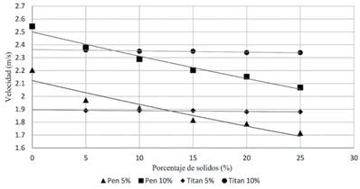
When representing the velocity results at the entrance of the curve, obtained from simulations in TITAN2F (Figure 3), we can see that the results for a 5% slope, with 5% and 25% of solids, are in a range between 1.89 and 1.88 m/s. For a slope of 10% and onwards, with the same percentage of solids, the range of the velocities are between 2.36 and 2.34 m/s.
When comparing with the values obtained in the laboratory, we observed that they are close to the mean velocities observed in the laboratory. However, the velocities measured in the laboratory have a greater range. In the case of a 5% slope, this range is between 2.2 m/s and 1.71 m/s for 0% and 25% of solids respectively. For a 10% slope, the range goes from 2.54 m/s and 2.06 m/s with 0% to 25% of solids respectively.
4. Discussion of results
4.1. Discussion o experimental results
As it was previously mentioned, a total of 420 tests were taken, 30 for each combination of variable, slope and percentage of solids, using averages for this analysis.
⍴𝑚 = ⍴𝑓 * (1- 𝜗𝑠) + ⍴𝑠 * (𝜗𝑠)
When graphing experimental velocity results and superelevation for a 5% and 10% slope, an approximately linear tendency can be observed (Figure 4), with the exception of data with 30% solids, which presented errors above 10%, which is why they are excluded from later analysis.
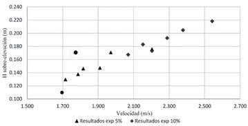
Figure 4 Experimental velocity results versus superelevation 5% and 10% slope. The Circles represent the data excluded from later analysis.
4.1.1. Velocity
For this analysis, we started by calculating the velocity of the flow at the entrance of the curve, using a Bernoulli approximation expressed by equation 6 3.
𝑉𝑏 is the velocity calculated at the entrance of the canal, ℎ1 is the height of the pile, 𝑠L is the slope of the bottom of the canal times the length of the path, ℎ2 is the height of the sheet at the end of the path and ℎ𝑓 the losses caused by friction, 𝑉𝑖 is the initial velocity of the flow. According to the initial laboratory conditions, ℎ1 is 0.2 m; ℎ2 is equal to 2.5 cm; ℎ𝑓 calculated by Darcy-Weisbach (equation 7) y (𝑉𝑖 2) is zero.
Where f is the friction coefficient calculated by Colebrook-White´s (equation 8) equation, L is the distinctive characteristic of the canal and Rh is the hydraulic radio, mean velocity of the flow.
Where ks is the rugosity coefficient, 𝕽 is Reynolds’ number.
The calculating of 𝑓 is carried out through an iterative process, ks is assumed as 0.0015 mm for the material of the artificial canal, and 𝕽 is determined by the mean velocity of the flow in the canal.
Basing ourselves in the hypothesis that there is a direct correlation between the calculated velocity from Bernoulli and the velocity observed at the laboratory, Equation 9 is postulated.
𝑉𝑐 = 𝐾*𝑉𝑏 (9)
Where 𝑉𝑐 is Bernoulli´s velocity, corrected so the density of the mix can be accounted for, and 𝐾 is the factor that relates 𝑉𝑏 and 𝑉𝑐. Taking into account that this factor must be equal to 1 for 0% of solids and it must diminish when increases the percentage of solids, it is assumed that 𝐾 is a function of the relationship of densities
When graphing the velocity and the density relations, Figure 5 shows that a different behaviour for each slope exists. Using linear regression, the experimental data was adjusted to equations 10 and 11.
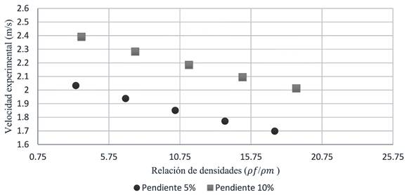
Figure 5 Relationship between velocity and the densities relation for 5 and 10 percent of slope, where (y) corresponds to the experimental velocity and (x) to the density relations.
Constants 2.136 and 2.51 of equations 10 and 11correspond to the calculated velocities for cero percentage of solids, using Bernoulli´s equation. In order to homogenize the mathematical model, a correlation between the exponents of equations 10 and 11 is made, with the longitudinal slope of the canal, and leaving the constants as the value of the velocity obtained with Bernoulli´s approximation (equation 6), thereby obtaining equation 12.
Where V
c
is the corrected velocity. V
b
is the calculated velocity of the flow, obtained from a Bernoulli´s approximation.
In order to verify the level of confidence of this equation, an analysis of Pearson´s linear correlation was carried out, obtaining coefficients r5% = 0.934 for a 5% slope and r10% = 0.985 for a 10% slope as a result 40. The number of Type t5 = 5.2639 and t10 = 11.4953 Deviations was calculated for the coefficients. These results were compared to the values in Student´s Table t, with a minimum confidence level of 95% and four degrees of freedom 41, which resulted in t (0.05, 4) = 2.78. This value allows us to conclude that the results that the equation predicts and the experimental data are correlated with a level of confidence of more than 95%.
4.1.2 Superelevation
In order to simplify the analysis of superelevation, equations 1 and 2 were equalized, thereby obtaining an equation where the width of the base is in function to the curvature radiuses (equation 13). This equation represents the condition that must be met so that a single equation of superelevation in function to velocity can be obtained. In the specific case of our canal the equation is achieved with a 0.9% of error.
By replacing the dimensions of the canal in equations 1 and 2, an equation of superelevation in function to the velocity can be obtained, which can be applied to fluids with no solids (equation 14). In the specific case of the canal, the equation presents an error of less than 1% when checked.
Taking into account that equation 14 is useful for pure water fluids, it is necessary to make an adjustment so that bi-phased flows can be accounted for. For this end, the differences between experimental data and the results from equation 14 (Figure 6) are calculated.
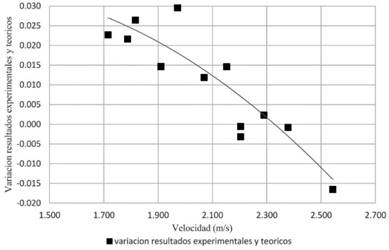
Figure 6 Difference between experimental and theoretical results. The continuous line represents the tendency of these results.
The difference between theoretical and experimental results on superelevation, which has been graphed above, shows a quadratic tendency, and the equation in function of the velocity (∆ℎ𝑐)
Was determined through minimum squares.
Where ∆ℎ𝑐 is the difference between theoretical results (equation 14) and experimental data.
The adjustment was made by adding equations 14 and 15. Taking the analysis of velocity, (equation 12) and it resulted in a superelevation equation, in function to the corrected velocity, which takes bi-phased fluids into account (equation 16).
Where ∆𝐻 is the superelevation that takes the percentage of solids into account.
Pearson´s factors for superelevation results are r5=0.97 and r10=0.95, thus, the Type Deviations result in t5=8.1 and t10=6.1, which shows that the experimental and theoretical results (equations 16) are correlated with a level of confidence greater than 95%.
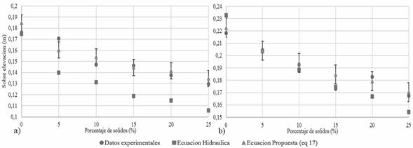
Figure 7 shows the relationship between superelevation and the percentage of solids, where the difference between the experimental results and hydraulic theory can be appreciated. This shows that the equations for superelevation are valid for pure fluids, but they do not allow a link to the percentage of solids in the flow.
4.2. TITAN2F results discussion
In regards to superelevation, when representing the results from TITAN2F in the GRASS GIS software (Figure 8), it can be seen how the simulation predicts a superelevation within the first 45 degrees of the curve just as it was observed experimentally. The height of the predicted for a 10% slope and 20% of solids is of 0.091m above the digital model.
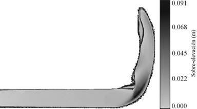
Figure 8 Ground layout representation of the GRASS GIS program in 1.3 seconds and a slope of 10% with 20% of solids.
It is important to take into account that the DEM´s resolution (1 cm) and the inclination of the walls of the canal, which is 60° in relation to the horizontal, generate an uncertainty of ± 3 cm vertically, which can explain part of the differences encountered.
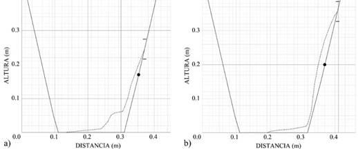
Figure 9 Comparison of the superelevation of TITAN 2F for a concentration of solids of 20% a) slope of 5% b) slope of 10%. The continuous line in a and b is the contour of the canal, the dotted line is the contour of the flow predicted by TITAN2F, the dot (*) is the superelevation measured in the laboratory and the range that has been marked at the end of the dotted line is the vertical uncertainty.
When graphing the cross sections where the simulation with TITAN2F predicts the superelevation phenomenon, it can be observed that for a 5% slope, the contour of this phenomenon is replicated by the program, as can be observed in Figure 9a. However, for a slope of 10% (Figure 9b), the contour shows a superelevation that is much bigger than the one observed in the laboratory, which allows us to conclude that when modelling in TITAN2F software, the slope has a bigger influence than the percentage of solids when defining the behaviour of the flow. When analysing superelevation results in these cross sections, an error of 28.87% and 48.85% for 5% and 10% slope, respectively, can be found. It is important to note that when increasing the slope to 10% (Figure 7b), it can be observed that the theoretical results come closer to the experimental results, based on the proposed standard deviation. However, the validity of the theoretical hydraulic equations continues to be deficient, especially for densities of over 20% of solids.
5. Conclusions
In this study, an experimental and numerical investigation for the superelevation phenomenon for the case of flows with sediments was carried out, where it was found that this phenomenon, when represented by the equations that hydraulics predicts (equations 1 and 2), shows an error of less than 5% for curve entrance velocity values between 2.0 and 2.5 m/s. When experimenting outside of this range of velocities, the percentage of error increases exponentially, which is why a correction was made in order to take the effect of the presence of sediments in the flow into account.
420 tests for 14 different scenarios were made. These tests were made with solid concentrations from 0% to 30%, with constant increases of 5%, however, it was observed that concentrations of solids greater than 25% in volume, presented a high degree of difficulty in mixing, which is why they were excluded from the analysis of results with 30% concentration of solids.
An analysis of the velocity was carried out and a new equation was formulated for the velocity of the flow. Taking the concentration of solids into account, this equation correlates the estimated velocity from Bernoulli´s energy equation and from a relation between the density of the fluid (liquid) and the density of the bi-phased fluid. The proposed equation (Equation 12 in this text) estimates a corrected velocity, inversely correlating the concentration of solids with Bernoulli´s approximation.
During the study, it was determined that an increase in the concentration of solids in bi-phased flows diminishes superelevation when transiting through the curve. Taking the results obtained in the laboratory into account, it can be observed that superelevation values calculated by hydraulics equations stray further than one standard deviation in results with a 5% slope. The error increases when more suspended solids are found in the mix. On the other hand, when making tests with a 10% slope, results for 5% up to 15% of solids in the mix are found within a margin of error of one standard deviation; results for 0%, 20% and 25% of solids go outside the margin of error with more than one standard deviation. superelevation results show us that hydraulics equations require an adjustment in order to the into account the concentration of solids in the flow, since their margin of validity is limited to 5%, 10% and 15% of solids with a slope at the bottom of the canal of 10%.
As for the analysis of the superelevation phenomenon, we made a statistical adjustment, obtaining a semi-empirical equation (equation 16), that adjusts the current mathematical model shown in equations 1 and 2 of the text to what was observed in the laboratory. Also, it was found that this phenomenon is also correlated inversely to the percentage of solids and is correlated directly to the velocity of the flow. It is important to mention that equation 16 is valid if the curve complies with the geometrical relation shown in this article (equation 13).
In order to verify the proposed mathematical model in this study, which is represented by velocity and superelevation equations, adjusted to bi-phased flows (equations 12 and 16), it was validated with Pearson’s lineal correlation method, from which confidence levels greater than 95% were obtained.
When carrying out a numerical modelling of the superelevation phenomenon with the experimentally analysed scenarios, it was observed that TITAN2F software generates the superelevation of the flow in the outer wall of the canal´s curve in the same way it was perceived experimentally. However, when a more detailed analysis was carried out, it was observed that the program shows low susceptibility to the increase in percentage of solids, in both velocities and superelevation. Also, it was found that superelevation shows a variation of 67%, which could be considered excessive with regards to the change in the slope.
Using the current version of TITAN2F and DEM software with a resolution of 1cm, a low susceptibility was observed for the increase of the percentage of solids. This is due to the fact that the program internally rounds the calculation values to one tenth of a millimetre, due to numerical requirements. This can mean that very small or very low-resolution canals are at the edge of the programs limit. In the same, the current DEM generate an uncertainty of 3 cm in the contiguous pixels of the canal walls, which can generate an error that is prolonged by rounding along the canal.
It should be noted that the results of this investigation are valid for prismatic canals, with surface conditions that are approximately smooth and with a curvature of 180°. Future investigations can be used in order to broaden and generalize results.

