


 English (pdf)
 Article in xml format
 Article references
 Send this article by e-mail
 Cited by SciELO
  Cited by Google
  Similars in
SciELO
Similars in
SciELO  Similars in Google
 Permalink
1. Introduction
Ray based technologies for radio propagation and channel prediction are taking a key role during last years, because of the deployment of OFDM based technologies like Long Term Evolution (LTE), LTE Advanced, DVB-T2 and WiGig (IEEE 802.11ac). Wireless technologies like MIMO must be fully developed to reach its maximum capacity in terms of speed and reliability. Consequently, it is imperative to know the environment where information is transmitted, that is, channel modeling. The main reason why ray based tools are resurging is that deterministic models delivers not only propagation losses information, but also channel parameters information.
Moreover, in indoor environments, an alternative to the traditional 2.4 GHz Wireless Local Area Network (WLAN) solution relies on the use of the 5.4 GHz band approved by FCC in the United States and considered by ITU. Generally, this last band presents better results in terms of data rate transmission and reliability in wireless communications either in the wireless network or in several devices, and is adequate for WiFi offload in 5G systems.
Given the high fidelity in physical simulations that game engines can offer and the advantages of GPU, together with their power for calculations, we now have solutions which improve computation time, using efficient ray tracing techniques implemented in game engines and combined with 3D design tools to implement the test scenarios.
Ray-Tracing and Ray Launching are deterministic techniques widely used for multipath channel parameters estimation. In general, ray based techniques whether Ray Tracing (RT) or Ray Launching (RL), are based on the seminal Works from Keller and Luebbers 1,2 about the application of Geometrical Theory of Diffraction (GTD) and Uniform Theory of Diffraction (UTD), in order to estimate the behavior of the radio wave in edges and wedges. These techniques were developed in ray based computer models (both RT and RL) in Works like Durgin and Cátedra 3,4, and has been evolving throughout the years. With recent developments in Graphic Processing Units (GPU) and the higher computational capacity, as well as the technical characteristics of current radio technologies like LTE and LTE-A, Digital TV (among others), ray based models has become relevant again, because of its ability to simulate not only propagation losses but channel parameters like delay and delay spread.
Ray based techniques are used to predict wireless channel parameters such as delay spread, Doppler spread, and angular spread in a variety of environments over a wide frequency ranges. In addition, Ray based techniques allows the characterization of the radio channel in temporal and spatial domains. Multipath channel model is the representation of a complex phenomenon that involves several mechanisms of interaction between the radio wave and the environment. Through Ray based techniques and multipath channel model, it is possible to design and, theoretically, evaluate wireless channels for 5G communication systems.
Accuracy of RT systems to estimate the multipath channel RMS-DS (Root Mean Square - Delay Spread) in indoor has been tested in different scenarios, frequency bands and communications services 5,6, but some recent papers have shown that, at microwave frequencies, when wavelength have only few centimeters, RT with diffuse scattering 7-9, because of walls rugosity, improves the accuracy for the calculation of RMS-DS, compared with the RT implementing only reflections, transmission and diffraction 5,6. Besides, has been observed that, at these high frequencies, RMS-DS is sensitive to the uncertainty of the constitutive parameters values, because of the building materials dielectric constants used or obtained for different frequencies 10,11.
However, at frequencies used for DVB-T2 in Europe and America’s countries using it, diffuse scattering does not have an important contribution to the RMS-DS, because the wavelength is big respect to the rugosity in indoor.
Technical specification for DVB-T2 (Digital Video Broadcasting) 12, incorporates OFDM (Orthogonal Frequency Division Multiplexing) modulation in order to improve spectral efficiency, and NGBT (Next Generation Broadcast Television) is analyzing the use of MIMO as an alternative to improve spectral efficiency and robustness in multipath channels 13.
Multipath propagation implies fading and the received signal can be attenuated and distorted by radio channel. The wave arrival using multiple paths produces ISI (Inter-Symbol Interference). Generally speaking, there are two different methods to reduce the effect of fading: equalization or diversity. However, in DVB-T2. As well as in many OFDM systems, a guard time was introduced, in order to protect against impulsive noise and time selective fading. For DVB-T2 the typical value for guard time is 70 m 12, but this time can be adjusted, as well as the equalization, in order to improve the performance of radio cannel. Other way, interaction between radio wave and distant obstacles may cause an excess delay higher than guard interval, causing ISI.
Therefore, in order to mitigate the effects of the frequency selective fading caused by multipath, the receiver need to perform a precise cannel estimation, and an efficient channel equalization. With the inclusion of the guard interval in DVB-T2, it is possible to cancel ISI, but it is necessary that the time spread of the channel be less or equal to the guard interval. Therefore, it is important to have simulation tools that allows to estimate the delay profile of the channel, like the one used in this paper.
In this paper, we use a ray launching tool (RL) based on 3D Game Engines, to simulate channel Delay Spread in a meeting room, in DVB-T2 frequencies. Simulation results are compared with measurements. One on the main limitations of deterministic propagation models is the need to have precise information of the simulated scenario; this means not only detailed information of geometrical characteristics of the scenario, but also an accurate information of the constitutive parameters of the simulated scenario (such as complex permittivity and conductivity). Values for such parameters depends on frequency as well as specific conditions like humidity, painting, etc. It is almost impossible to have precise information for any material in any frequency and condition, which incorporates an error factor in any deterministic simulation tool.
Generally speaking, it is not easy to find parameters’ values for different materials, but for the frequency band used in this work is even more difficult, because most publications reports values for higher frequencies, like the ones used in cellular systems.
The main goal of this paper is to compare and adjust complex dielectric values for the different materials in the scenario, using measurements in DVB-T2 band in an indoor scenario, using a 3D RL simulation tool, obtaining RMS-DS.
The paper is organized as follows: in the next section, the 3D model of the scenario is shown; then we explain the 3D RL model used for simulations, the scenario and the measurement procedure. Section 4 shows results. Finally, conclusions.
2. 3D Model of the scenario
In 3D indoor models for ray launching, one important issue is modeling the environment with all the objects present in it and their features. Also, these objects must be modeled with a high geometric resolution representation of the indoor scenario. In addition to that, to achieve accurate results using RT techniques, it is necessary to represent the electromagnetic characteristics of the different materials in the scenario.
Figure 1 shows 3D model of the iTEAM (Instituto de Telecomunicaciones y Aplicaciones Multimedia) meeting room at Valencia Technical University in Spain, used for the simulations and measurements. The 3D model of scenario was developed using 3D tool Blender. This included all elements presents in the realistic scenario. We used planar geometries for represent each object achieving great 3D resolution in the model. This was exported from Blender to an XML format, then the archives were imported in the game engine Jmonkey, in order to apply RT techniques using the Game Engine and GPU. The simulated and analyzed scenario is a conference room in a University. The scenario has dimensions of 7.16x7.62x2.64m.
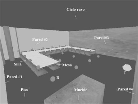
Seven different materials were identified in the scenario. We store and manipulate the constitutive parameters information as an attribute within the 3D Model (i.e. permittivity). According to their electromagnetic material properties, the floor, ceiling, desk, windows, chairs, wallboard, column, VNA, video beam, lamp and structures of windows, desk, and chairs, were classified into 5 different classes of dielectric material parameters. Nevertheless, all these materials are assumed to be homogenous and their material properties at DVB-T2 frequency band are summarized in Table 1. Darker spheres are the measurement points and the lighter sphere with T letter is the transmitter.
Table 1 Initial value for relative permittivity and conductivity.
| Element | Material | Initial Group | Relative Permitivity | Conductivity (S/m) |
|---|---|---|---|---|
| Floor and ceiling | Concrete | Concrete | 6.9 | 0.0138 |
| Walls #1 y #2 | Metallized glass | Metallized glass | 2.4 | 0.0350 |
| Table | Glass | Glass | 2.4 | 0.0350 |
| Walls #3 y #4 | MDF | MDF | 20.0 | 0.0200 |
| Furniture | Wood | Wood | 3.81 | 0.0070 |
| Chair | MDF | MDF | 20.0 | 0.0200 |
We use Ray Launching techniques combined with 3D model of the scenario, implemented in Game Engines and GPU. Previous works of the authors shows that this techniques are appropriate to estimate with high precision and small processing time multipath channel parameters 11,14-17.
The initial values used for the permittivity and conductivity of the materials present in the scenario were found of the literature 18. We assume initially the same values for permittivity, assuming dielectric behavior and later we adjust parameters, according to simulation results. Different materials were grouped initially in six different groups, according to its characteristics: concrete for floor and ceiling; glass for the table, metalized glass for walls #1 and #2; wood for the furniture; MDF for the chairs and walls #3 and #4; metal for columns. This grouping has the aim of obtain initial values of dielectric constant whose values are not known, but is possible to use values from similar materials. Nevertheless, all these materials are assumed to be homogenous and their material properties at DVB-T2 band are summarized in Table 1.
Diffuse component is defined as the dispersed signal in different directions because of the rugosity of the Surface 13. In order to obtain the diffuse component because of the rugosity of the walls in the scenario, we made a literature search to find the rugosity value for concrete, finding a value of 1mm for concrete and 0mm for glass and wood walls.
Rugosity factor for a Surface is expressed as:
Being θ i the incidence angle, δ the rugosity factor and λ the wavelength.
In (Eq. 1) it can be noted that the rugosity factor depends on the cosine of the incidence angle θ i , as well as the rugosity factor δ and the wavelength λ, expressed in the parameter δ/λ. For the case of DVB-T2, the parameter is less than 1, therefore the scattering is negligible and was not included in the simulations.
3. 3D RL model and simulation
3.1 Ray launching simulation parameters
Simulation was performed with a 3D Ray Based software using GO (Geometrical Optics) and UTD (Uniform Theory of Diffraction) 14, implemented on an Open Source Game Engine. Radio waves are modeled as an optic ray that follows a straight path from the transmitter to the receiver. During this process, the wave interacts with bounding boxes for flat objects, bounding spheres for receivers and bounding cylinders for edges. Initially, we only processed reflections, diffractions, free space attenuation, and multiple combinations of these effects. In order to model walls, floor and roof reflections, we apply Fresnel coefficients.
The RL algorithm used is the shooting and bouncing launching algorithm (SBR) 3, which is based on launching a ray from the transmitter to the antenna and verify if the ray impacts on a wall or edge. The mean angular separation between neighboring rays in 3D space used for rays launched is 0.26°.
The implemented algorithm is limited to 10 events, defining an event as a reflection, diffraction or transmission, and a maximum value of two diffractions at vertical or horizontal object edges, which is appropriate for outdoor environments. We use the computational capability of the graphics card to estimate where the ray might hit with all possible bounds present in the model.
In our model, if the ray hits an edge, the resulting rays of first and second diffraction cone will be computed with a given angle increment. It is considered that, for the first diffraction cone, the angular resolution fixed in the 3D space for diffracted generated rays α e . Likewise, 2α e is the angular resolution for the second diffraction cone, assuming that the resolution of the diffracted rays decreases according to their order. This reduces dramatically the memory and processor usage without any significant loss in the prediction accuracy if a high initial resolution of α e is adopted.
At each interaction of the ray with an obstacle, the field strength is multiplied with a dyadic propagation transfer factor, which accounts for the actual propagation effect and for a change in divergence due to the interaction event: diffraction, transmission or reflection.
Figure 2 shows the path obtained with the simulator, between the transmitter (lighter sphere) until its impact in the receiver (darker sphere). It can be noted that the ray experiments a total of 6 interactions in the path between transmitter and receiver, represented by 𝑛 = 1,…,N(𝑡) paths (Eq. 1).
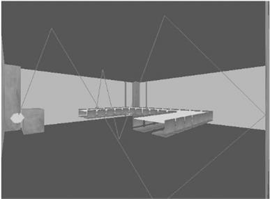
Figure 2 Path of a successful ray between transmitter (lighter sphere) and measurement point (dark sphere).
To estimate parameters of multipath propagation due to reflections and diffractions is necessary to distinguish inherently between individual propagation paths. The SBR algorithm is particularly suitable for this task. The most important channel characteristics can be estimated obtaining path parameters based on the frequency response 𝐻(𝑓, 𝑡) and the time-variant channel-impulse response of the channel ℎ(𝑡, τ).
The path parameters for the propagation between the transmitter and the receiver is defined by n = 1,…,N(t) propagation paths. The identified propagation parameters between the transmitter and the receiver are:
τ(𝑡): time delay of arrival (TDA) of path ;
Ω T, (𝑡): direction of departure (DoD) of path ;
Ω R, (𝑡): direction of arrival (DoA) of path .
Cascading all transfer factors (and therefore all occurring propagation phenomena) leads to the full polarimetric transmission matrix
The low-pass impulse response of the channel ℎ(𝑡, τ) is obtained by the inverse Fourier transform of (Eq. 1).
Where is the speed of light in vacuum and 𝑓𝑐 is the center frequency of the system represents the complex amplitude of the multipath component and incorporates the properties of the transmitter and receiver antenna. Thus, the channel model could be represented as a power delay profile (PDP) as the summation of the received power of each multipath component 17 and expressed by:
RMS-DS is obtained from (3) and is defined by:
Being (τ 𝑘), the power of each path and τ 𝑘 is the delay of each path.
3.2 Measurement campaign
Measurement campaign was executed in a meeting room with 10m by 6m with typical furniture: Table, chairs, carpet and walls of soft materials. Outside the windows, above the ceiling and below the floor, we found steel, quite common in the constructive techniques used in the last 15 years. Ceiling and floor use the system known as steel deck. Outside the windows, we found some steel bars and metalized glass.
These characteristics of the constructive elements causes reflection effects that can increase the number of reflections to be considered in the model. We show the measurement scenario modeled in 3D tool, indicating the walls, ceiling, floor, table and chairs. Measurement points are shown as dark spheres. The receiver points were located at 1m distance between them, for a total of 39 points in the scenario. Lighter sphere in the figure corresponds to the transmitter and is marked with a T. The transmitter is located 05m away from the wall #4 and is centered between walls #1 and #3. Height from the floor for transmitter and receivers is 0.9 m.
Measurement campaign was carried out by the iTEAM research institute inside Building. Measurements were taken using the iTEAM’s Rhode & Schwarz ZVRE. Receiver antenna is a PROCOM vertically polarized, with 2 dBi gain; the operation frequency was 594 MHz and RF power was 10 mW. We store and manipulate the constitutive parameters information as an attribute within the 3D Model (i.e. permittivity). VNA was located outside the scenario, in order to avoid include it in the 3D model. People making measurements also were located outside, to keep stationarity of the channel According to their electromagnetic material properties, the structures of the walls, floor, table, windows and chairs were classified into 5 different classes with dielectric material parameters shown in Table 2. Values for conductivity are shown in Table 2. We assume initially the same values for conductivity, assuming dielectric behaviour and later we adjust conductivity parameters, according to simulation results. Using the S parameters delivered by the measurement system, we estimate the Delay Spread values, which are compared with simulation results.
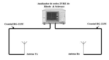
Table 2 Adjusted values of relative permittivity and conductivity.
| Element | Material | Initial Group | Real relative Permittivity | Conductivity (S/m) |
|---|---|---|---|---|
| Floor and ceiling | Concrete | Concrete | 6.9 | 0.0138 |
| Walls #1 and #2 | Metallized Glass | Metallized Glass | 2.4 | 0.125 |
| Table | Glass | Glass | 2.4 | 0.0350 |
| Walls #3 y #4 | MDF | MDF | 60 | 0.02 |
| Furniture | Wood | Wood | 3.81 | 0.007 |
| Chairs | MDF | MDF | 70 | 0.02 |
A similar work, but at different frequency was reported 13, showing a similar behavior for constitutive parameters. However, the paper of Vitucci et al. does not describe measurement process or simulated frequencies, making difficult to compare the results with this paper. One of the relevant aspects of the mentioned work are the effects of the external metallic structure over channel delay values, resulting in bigger measured values than simulated ones, given that the authors does not include the external metallic structure in the scenario model.
3.3 Complex dielectric constant adjustment
Since the beginning of the process, we use uncertain permittivity and conductivity values, because was based on information from literature for different frequencies, and it is well known that constitutive parameters’ values change between materials with frequency, humidity and a lot of variables, leading to a huge challenge to deterministic models, related to the adjustment of constitutive parameters 19. Because of that, the main objective in this work is to discuss the adjustment process of constitutive parameters in ray based models.
For materials with real permittivity and real conductivity 18, complex permittivity ε can be written as:
Where ε 𝑟 represents complex relative permittivity, ε r ′ represents real relative permittivity, ε r ′′ relative imaginary permittivity, σ conductivity in 𝑆/𝑚, ⍵ is the frequency in rad/s and ε 0 is the value of vacuum permittivity, equals to 8.85x10⁻¹² F/𝑚.
For dielectric materials with low losses, usually it is assumed that conductivity value is included in the ε r ′′ value and the conductivity is assumed zero. Then complex permittivity can be written as:
Recent literature shows that for low complex permittivity values as shown in (Eq. 8), the RMS-DS has a high sensitivity to the ε r ′ value, but is less affected by the uncertainty value of ε r ′′ (Eq. 7). For dielectric materials with a conductivity has a bigger value compared with ε r ′′, we can assume that it is included in the conductivity term, and complex permittivity from (Eq. 7) can be written as:
In order to adjust complex permittivity for materials with uncertainty in the values, we adjust the values for ε r ′ and σ in (Eq. 9), to analyze the impact on RMS-DS.
For adjustments, we assume that random variables describing real and imaginary parts of complex dielectric constant are independent between them. This assumption is based on Kramers-Kronig 20 relations for narrow band channels. With this assumption for (Eq. 9), when we analyze the impact of ε r ′ over the simulation results, we assume σ as constant and vary the values of ε r ′. A similar argument is used to analyze the impact of σ over the simulation results.
In order to improve RMS-DS prediction values, we adjust the values for ε r ′ and σ for each one of the six materials, excluding metallic columns from the analysis.
In order to analyze how the predictions are affected by the simulated objects characteristics, we assumed a set of values for each of the classes and by changing one of these values at a time, the model’s sensitivity to that parameter is evaluated. First, delay spread results are examined for the varying values of permittivity for one class within range from -10% to 10%, in steps of 1 at processing time. Second, using this method reiteratively, we obtain the global minimum standard deviation for best values of each class for all the above predictions, respect to the measurements.
4. Results and analysis
In Figure 4 we show the RMS-DS measured values (gray line with squares) and estimated values using RL (black line with circles) using the initial values for ε r and σ shown in Table 1. It can be observed that RMS-DS values for the 39 points have important differences respect the measured values. Besides, as shown in Table 3, for the initial simulation the mean error and the standard deviation are 10.7 ns and 21.6 ns respectively, indicating low precision of the RL, respect to the mean value of the RMS-DS of 14.5 ns.
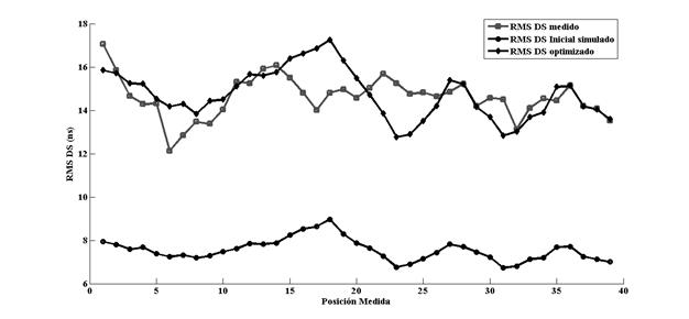
Figure 4 RMS-DS measured (light gray with squares), RT before adjust (black with circles) and adjusted (black with rhombs).
Table 3 Error statistics comparison.
| Process | Standard Deviation (ns) | Mean error (ns) |
|---|---|---|
| Initial | 21.6 | 10.7 |
| After Adjustment | 1.1 | 0.1 |
The impact of RMS-DS error was analyzed when the permittivity was modified for each of the materials, but keeping conductivity values unchanged. Same procedure was applied to the conductivity, keeping values of permittivity. In Figure 4 we show the results of the simulation after the permittivity adjustment, using the black line with rhombs. , The main impact was found in the values of permittivity for walls #3 and #4 (MDF), chairs (MDF covered with fabric), and the conductivity for walls #1 and #2 (metallized glass with metallic frames). These materials had an important effect in the results of the simulated RMS-DS, after the adjustment of the relative permittivity and conductivity, as shown in Figure 4. For the remaining of the materials, the impact was negligible. Adjusted values of relative permittivity are: εr′= 60 for MDF (walls) and εr′= 70 for MDF with fabric cover, and are shown in bold in Table 2.
Results for estimated values of RMS-DS after modify the conductivity of the rest of material are not shown, because its impact is negligible. The value for adjusted conductivity is 𝜎= 0.125 S/m and is shown in bold in Table 2.
In Table 3 it is observed that after adjust the conductivity for walls #1 and #2 mean error reduces to 0.1 ns and standard deviation to 1.1 ns. These results shown that the adjust of the conductivity in walls #1 and #2, may lead to better results than just adjust the real relative permittivity.
It is important to remark that, even after the adjustment of both permittivity and conductivity in walls #1 and #2, there still exist some important differences in the results of the Delay Spread. A similar work recently published 21 found that the influence of external structures highly conductive, like metallic frames from the building structure, can reflect the waves, generating high values of delay, explaining the existing differences. These factors were not considered when we execute the measurements, then, it is not possible to validate such hypotheses at the moment of writing this paper.
5. Conclusions
Ray based tools are very accurate to predict the behavior of the radio cannel, even for low frequencies like the used for this paper. However, and as has been shown, these tools are quite sensitive to some parameters, like materials constitutive parameters and the scenario.
For the new frequency bands, identified by the WRC-15 for 5G mobile technology, ray based models are more relevant, as well as constitutive parameters information.
The empirical adjustment of constitutive parameters shown in this paper is a contribution to the discussion about how deterministic are really the ray based models, or about the tradeoff between deterministic part and empirical part of the models.
Measurements were done in the year 2012, and since then some papers has been published in mmWave bands (above 6 GHz) using ray based models, it is important to execute more measurements in these mmWave bands, and also to consider the metallic structures of the building in the simulated scenario.

