


 Inglês (pdf)
 Artigo em XML
 Referências do artigo
 Enviar este artigo por email
 Citado por SciELO
  Citado por Google
  Similares em
SciELO
Similares em
SciELO  Similares em Google
 Permalink
1. Introduction
Stage - discharge rating curves in a river define or establish the relationship between stages or water levels (H) and discharges (Q) and are very useful because they allow estimating discharge flows using level records in a hydrometric station. These curves can be simple or complex depending on the flow regime and the characteristics of the stretch of river under study. Most of the rating curves are simple and to determine them gaugings data are required (water levels and discharges). Numerous studies can be found in the literature for the determination of rating curve considering different methods (graphs, statisticals, neural networks, etc.) and their extrapolation for high water levels (due to the difficulties and risks inherent to the measurements for these conditions) 1-4. Schmidt and Yen 5 examined the relationships of rating curve in open channels based on the basic hydrodynamics of non-uniform non-steady flow and identified terms in the Saint-Venant equations that should be considered in the rating curves. León et al. 6,7 derived the level - discharge relationship of 21 virtual measuring stations in the River Negro (Amazon), using satellite altimetric measurements; the discharges were calculated using a routing discharge model based on Muskingum - Cunge.
When there is a non-stationary regime (due to the operation of a reservoir upstream, for example) or when the slope of the free surface of the water is variable (due to the backwaters produced by discharges of a tributary located downstream or due to a reservoir) there is no simple relationship between levels and discharges, so a complex rating curve must be established 8. In this case, discharges must be related to water levels and another additional variable, such as the rate of variation in water levels in a gauging station or the slope of the free surface of the water. Authors such as Kennedy 8, Aldana 9, Lohani et al. 10, Sadeghi et al. 11 and among others, describe methods for determining complex rating curves. Bhattacharya and Solomatine (1), Ajmera and Goyal 12, Kashani et al. 13 and Zeroual et al., 14 use artificial neural networks in the estimation of this type of curves.
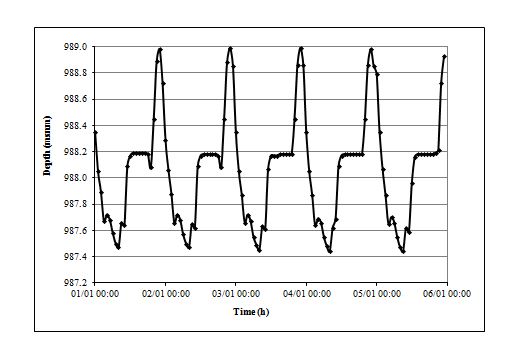
The operation of the Salvajina reservoir for power generation imposes most of the time a very dynamic regime in the Cauca river, causing downstream discharges higher than those of the steady state when the water level rises and lower when the water level drecreases (CVC - Universidad del Valle, 2000). This produces a storage in the section that causes a loop in the Level - Discharge relationship, which is a phenomenon known as hysteresis. Based on the available field information in the Corporación Autónoma del Valle del Cauca, CVC, in the period 1999-2004, simple and complex rating curves were determined and compared with each other in the La Balsa station, located about 27 km downstream of the Salvajina reservoir 15. In this gauging station the river has an approximate width of 65 m and a depth to bank full of almost 3.5 m, the slope of the left bank is pronounced and that of right margin relatively smooth 16; During the gaugings, which are carried out by suspension from a cable car, a rapid variation of river levels is presented due to the regulatory effect of the Salvajina reservoir (Figure 1). Discharges were calculated for flood of January 01 of 1999 using simple and complex rating curves, with differences of up to 19% between the estimated discharges using each of these curves. Several authors have examined the uncertainties in the rating curves and uncertainties resulting from discharges records 17-20 Petersen and Reitan, 2008.
The study was developed following and applying the methods and procedures of the ISO Standards for the elaboration of rating curves Level - Discharge (21,22) and the Techniques of Water Resources Investigations of the U. S. Geological Survey 8. as well as other national and international guides. 9,23.
2. Methodology
2.1. Simple rating curve
Simple rating curves, the most common in practice, relate discharges only to stages in a hydrometric station, in steady or permanent regime. This relationship can be determined after making numerous measurements of levels and discharges covering a wide range of levels to define a continuous curve. There are different methods for the elaboration of simple rating curves, such as: graphic, hydraulic equations (Manning and Chezy) and analytical (logarithmic, parabolic and the three curves). In the hydrometric stations of the Cauca River (Reach Salvajina - La Virginia), simple rating curves were determined considering all these methods 15 and no appreciable differences were found between them.
In this study, the logarithmic method was adopted to determine the simple rating curve because it has the following advantages: (i) it allows identifying the type of control (section or channel) that determines the relationship Stage - Discharge for a certain range of levels ; (ii) in a logarithmic scale graph it is easier to establish if the control type changes from a certain level and, therefore, to determine with better approximation the shape, curvature, position and tendency of the rating curve for the different ranges of levels; (iii) it allows plotting transition curves in those ranges where changes occur in the types of controls; and, (iv) it allows establishing the effective level of zero discharge.
If the section of a river can be approximated to a known geometric figure, the discharge in the section can be expressed as:
where: Q = discharge (m3/s), H = measured water level (m), H0 = effective level of discharge zero (m), C = coefficient (constant), n = exponent (constant).
This expression is equivalent to the following equation:
Which represents the equation of a straight line of slope n and intercept Log C.
The effective level of discharge zero (H0) is the water level that, when it is subtracted of the water levels obtained during gaugings, will produce a straight line in the relation Level - Discharge in a logarithmic scale graph 22. Generally H0 is not known and can be found by trial and error, assuming different values of H0 and plotting Log Q vs. Log (H-H0); the final value of H0 is the one that allows obtaining the best fit to a straight line. Statistically, the correct value of H0 will be the one for which the coefficient of determination of the regression is maximum. The measured water level minus the effective level of discharge zero represents the effective depth of flow in the control (H-H0).
2.2. Complex rating curve
The Stage - Discharge relationship can be affected by different circumstances and events. An existing reservoir downstream of a hydrometric station can originate backwaters upstream, and to submerge totally or partially the flow control of the station and, therefore, to invalidate the Level - Discharge relationship. Likewise, a tributary discharging downstream or within the flow control section of the station can generate variable backwaters in the main channel, which can submerge the control and affect the stage - discharge relationship. Also, the operation of a dam for purposes of energy generation imposes conditions of dynamic or non - stationary regime downstream in the river, resulting in an effect known as "hysteresis" or "loop curve". Different authors, such as, Lohani et al.10, Braca 24, Sadeghi et al. 11 and Birgand 25 deal with this phenomenon. When the water levels rise, an accelerated flow occurs and the velocities and discharges are higher; on the other hand, when the levels decrease, there is a deceleration of the flow that reduces the velocity of the water. Therefore, the actual discharge for a given water level will be greater than the "normal" discharge (taken from the simple rating curve) when the water level rises and the actual discharge will be lower than the "normal" discharge when the water level decreases. In all these cases, in which the free surface of the water and its gradient are variable and there is no simple relationship between the levels and the discharges, complex rating curves must be developed.
A calibration loop can be plotted by joining the consecutive discharge data during a flood. If the complex rating curve has already been established, the loop for each flood can be obtained (without discharge measurements) by joining the successive points of instantaneous levels and the corresponding calculated discharge of that curve. Generally, two types of auxiliary curves are used in the determination of the rating curve: (i) H vs. ΔQ / J (effect of storage by rate of variation in the level), which treats the loop of the rating curve as a simple storage phenomenon; and (ii) H vs. 1 / USc, which considers the magnitude of the loop to the velocity of the flow waves (U) and to the slope of the water surface at constant discharge (Sc). This last method was not applied in the La Balsa station, because there is no auxiliary topographic stadia rod near the station that allows determining the slope of the free surface of the water.
Method of storage per unit of water level variation rate (ΔQ / J)
The main components in this method are a Level - Discharge curve for steady regime and a storage curve. The actual discharge is calculated by adding a correction per storage to the discharge obtained from the Level - Discharge curve for steady regime. The storage correction is the value obtained from the storage curve multiplied by the rate of change in the water level. The equation to determine the discharge in non-steady regime is the following:
where: Qm = Measured discharge, Qr = Discharge read from the rating curve, ΔQ = Difference between the actual discharge measured and the discharge read from the rating curve, J = Rate of variation in the water level during the gauging.
The method of variation rate of water level does a correction of the discharge in the river in accordance with the storage that occurs during a flood. This correction is achieved by constructing two curves: a Level - Discharge curve for steady regime condition and an auxiliary storage curve level - ΔQ / J.
The rating curve is obtained by trial and error, starting with a curve plotted very close to the measurements made during the condition of steady or quasi- steady regime. The difference between each measured discharge and the discharge read of the previous curve for steady state (ΔQ) is divided by the rate of change in the water level during the gauging (J) and plot against the water level in another graph. The storage curve represents the storage correction due to the variation rate over time of the water level and is based on these plotted points. Each measured discharge is adjusted to steady regime conditions (corrected by storage effect) using the storage curve. The process is repeated until refinement of the rating curve or storage curve is not possible.
The curve ΔQ / J must be plotted by giving different weights to the plotted points [(Qm - Qr) / J]. Those points based on measured flows, whose rates of variation in water levels during gauging (J) are high have a greater weight and, therefore, the storage curve should be plotted close to those points.
The general shape of the storage curve ΔQ / J is predictable. Generally the storage curve starts with a value ΔQ / J equal to zero for the water levels where the control of low waters is submerged, it increases until reaching a maximum value at a level close to bankfull and again it becomes zero when the flow above the bank contains more than half of the discharge. The curve should be as gradual or smooth as the data allow.
The procedure to determine the complex rating curve is as follows:
1. Prepare the field data and tabulate the following information: indicator or number of the gauging (Column 1), measured water level (H, Column 2), gauged discharge (Qm, Column 3) and hourly change rate of the water level during the gauging (J, Column 4).
2. Graph the field data of Water Level against Discharge in log-log paper.
3. Plot a first curve Level - Discharge: the curve must be plotted very close to the points corresponding to the steady regime, to the left of the gaugings carried out during the ascending water levels and to the right of the descending water levels. Then skip to step 6 for the first calculation or trial.
4. Graph the data of level against the adjusted discharge (Qaj) (recorded in Column 10).
5. Plot the curve Level Vs. Adjusted Discharge: this curve must average the points plotted in point 4, as much as possible.
6. Read the discharges values of the curve plotted in step 3 (first trial) or in step 5 (subsequent trials). These discharges are recorded in Column 5 (Qr)
7. Calculate and record it in Column 6 ΔQ = Qm-Qr, that is, subtract Column 3 minus Column 5. If 0.03> J> -0.03 (m / h), write a hyphen (-).
8. Calculate and record in column 7 the values of ∆Q/J: If a hyphen (-) was entered in column 6, also write a hyphen (-) in column 7; Otherwise calculate ∆Q/J, i.e., divide the values of column 6 (∆Q) between the values of column 4 (J).
9. Graph the Water Level data (H, Column 2) against the values of ΔQ/J (Column 7) on a log-log paper. Use a different symbol or convention for points corresponding to high values of ΔQ/J.
10. Plot the Storage Curve, i.e., Water Level Vs. ΔQ/J: the storage curve must be very close to those points corresponding to high values of ΔQ/J. The maximum value of ΔQ/J is generally just above the bank full level of the channel section; ΔQ/J is zero when the section control is effective and again when the floodplain contains most of the total discharge.
11. Read from the storage curve (Level Vs ΔQ/J) the values of ΔQ/J and register them in Column 8 (ΔQ/J) aj
12. Calculate and record in Column 9 the new values of ΔQ (now called ΔQaj) for all measurements (regardless of the magnitude of J), as follows:
13. Calculate and record in Column 10 the adjusted discharges as follows: Qaj = Qm - ΔQaj; i.e., subtract columns 3 and 9.
14. If the two Level-Q and Level-ΔQ/J curves cannot be improved, continue with step 15. If an additional trial is required, return to step 4.
15. Calculate and record in column 11 the relative difference (Rel. Dif.) Between the adjusted discharge (Qaj) and the read discharges (Qr) according to the expression:
If the relative differences are acceptable, continue with step 16; otherwise, perform a new test by returning to step 4.
16. Final test: With the data of the measured water levels during a flood in the river, calculate the corresponding discharges. If the H-Q curve of the flood (loop) is reasonable, then the curves H-Q and H-ΔQ/J will be the last ones plotted. Otherwise, a new trial must be carried out by returning to step 4.
Calculation of discharge based on the complex rating curve (water level variation rate method)
Tabulate the hourly water level data, including date and time.
Calculate the value of the variation rate of levels (J) for each water level data. It must be taken into account that:
J> 0 when the Water Level is rising (ascending phase of the flood) and
J <0 when the Water Level is downing (descending phase of the flood)
From the auxiliary curve (Level vs ΔQ/J) read the value of (ΔQ/J)aj for the corresponding Level.
Calculate the value of ΔQ, according to the following expression: ΔQ = (ΔQ/J)aj * J
For each level value read the corresponding discharge value (Qr) of the rating curve plotted for steady regime.
Finally, the discharge (Qm) for a given water level will be the discharge read from the rating curve (Qr) for steady regime plus ΔQ (Eq. 3).
3. Results and discussion
3.1. Simple rating curve
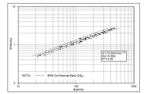
Figure 2 shows the simple rating curve obtained for the La Balsa station. It is observed that the slope of the line, which represents the exponent of (H-H0), is less than 2.0, which indicates that there is a channel control for the H-Q relationship; i.e., the relationship is determined by the characteristics of the stretch of the river downstream of the station, such as roughness, slope and shape and size of the section of the main channel.
3.2. Complex rating curve
In order to generate the rating curves, the existing gaugings from 1999 to 2004 in the different hydrometric stations were considered. In La Balsa station there are gaugings records carried out during the ascending and descending phases of floods, as well as in steady state conditions; this allowed calculating the corresponding complex rating curve. Generally, the fluctuation of the water level during gaugings is important.
Table 1 shows the calculations made to determine the complex rating curve in La Balsa station through the Water Levels Variation Rate Method. Because it was not possible to refine the Q-Level and ΔQ/J curves, no additional tests and calculations were carried out to those presented in the Table 1. As shown in this table, the number of field records available for the ascending and descending phases of floods is limited. Having a greater number of data for these two conditions, it will be possible to achieve a better adjustment of the Level-Discharge curve and the auxiliary curve Level-ΔQ/J and, therefore, a lower uncertainty in the discharge deduced from the water levels measured in field. Figure 3 shows the Level-Discharge curve and the auxiliary curve Level-ΔQ/J finally found. Table 2 shows the calculated discharges for the moderate flood of January 01 of 1999.
3.3. Simple curve vs. complex curve
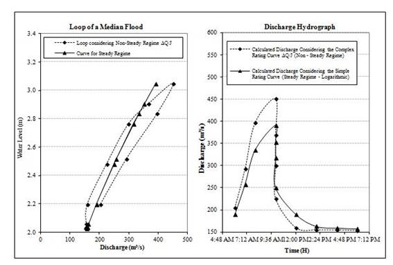
To illustrate the differences that can occur in the estimated discharges, the two rating curves found (simple and complex) were applied for the moderate flood of January 01, 1999. In the hydrographs obtained (Figure 4), it is observed that when the simple curve (steady state) is used during the ascending phase of the flood the discharges are underestimated (with respect to the real situation, i.e., using the complex curve), and when the water levels descend the discharges are overestimated. For the evaluated flood, the calculated discharge using the two rating curves obtained can differ up to about 19%. For more intense floods the differences could be greater.
Table 1 Determination of the complex rating curve through the water level variation rate method (ΔQ / J). Station: The: La Balsa
| Column 1 | Column 2 | Column 3 | Column 4 | Column 5 | Column 6 | Column 7 | Column 8 | Column 9 | Column 10 | Column 11 |
|---|---|---|---|---|---|---|---|---|---|---|
| Gauging No. | H (m) | Q m (m 3 /s) | J (m/h) | Q r (m 3 /s) | ΔQ (m 3 /s) | ΔQ/J (m 3 /s/m/h) | (ΔQ/J) aj (m 3 /s/m/h) | (ΔQ/J) aj *J (m 3 /s) | Q aj (m 3 /s) | Rel. Dif. (%) |
| 1 | 1.04 | 23.65 | -0.09 | 27.55 | -3.90 | 42.62 | 31.00 | 2.84 | 26.49 | 3.86 |
| 2 | 1.03 | 23.42 | -0.14 | 26.87 | -3.45 | 25.16 | 30.00 | 4.12 | 27.54 | 2.47 |
| 3 | 1.15 | 33.87 | -0.05 | 35.69 | -1.82 | 34.73 | 35.00 | 1.83 | 35.70 | 0.04 |
| 4 | 1.42 | 52.01 | -0.18 | 61.38 | -9.37 | 53.09 | 47.00 | 8.30 | 60.31 | 1.75 |
| 5 | 1.27 | 51.93 | -0.13 | 46.53 | 5.40 | -41.26 | 42.00 | 5.49 | 57.42 | 23.40 |
| 6 | 1.43 | 56.12 | -0.20 | 62.50 | -6.38 | 32.52 | 47.50 | 9.32 | 65.44 | 4.70 |
| 7 | 1.96 | 120.10 | -0.26 | 141.41 | -21.31 | 81.49 | 63.00 | 16.48 | 136.58 | 3.42 |
| 8 | 2.51 | 236.93 | -0.30 | 266.46 | -29.53 | 98.19 | 78.00 | 23.46 | 260.39 | 2.28 |
| 9 | 1.54 | 83.78 | 0.49 | 76.24 | 7.54 | 15.28 | 51.00 | -25.15 | 58.63 | 23.11 |
| 10 | 1.70 | 100.21 | 0.09 | 97.47 | 2.74 | 29.88 | 55.00 | -5.03 | 95.18 | 2.36 |
| 11 | 1.67 | 109.82 | 0.08 | 93.83 | 15.99 | 203.74 | 54.00 | -4.24 | 105.58 | 12.52 |
| 12 | 1.62 | 111.64 | 0.26 | 86.12 | 25.52 | 96.37 | 53.00 | -14.03 | 97.61 | 13.34 |
| 13 | 2.42 | 256.80 | 0.37 | 242.67 | 14.13 | 37.92 | 75.00 | -27.95 | 228.85 | 5.70 |
| 14 | 2.57 | 318.02 | 0.20 | 283.08 | 34.94 | 173.16 | 81.00 | -16.34 | 301.68 | 6.57 |
| 15 | 1.00 | 21.38 | 0.00 | 25.23 | - | - | 29.80 | 0.00 | 21.38 | 15.25 |
| 16 | 1.05 | 28.20 | 0.00 | 28.59 | - | - | 31.01 | 0.00 | 28.20 | 1.35 |
| 17 | 1.37 | 56.59 | 0.00 | 56.50 | - | - | 46.20 | 0.00 | 56.59 | 0.15 |
| 18 | 1.54 | 83.94 | 0.00 | 76.24 | - | - | 51.00 | 0.00 | 83.94 | 10.09 |
| 19 | 1.56 | 87.92 | 0.00 | 78.16 | - | - | 51.30 | 0.00 | 87.92 | 12.49 |
| 20 | 1.56 | 89.59 | 0.00 | 78.81 | - | - | 51.30 | 0.00 | 89.59 | 13.68 |
| 21 | 1.61 | 90.98 | 0.00 | 84.76 | - | - | 53.00 | 0.00 | 90.98 | 7.33 |
| 22 | 1.60 | 92.59 | 0.00 | 84.09 | - | - | 52.00 | 0.00 | 92.59 | 10.11 |
| 23 | 1.99 | 113.13 | 0.00 | 146.08 | - | - | 64.00 | 0.00 | 113.13 | 22.56 |
| 24 | 1.95 | 115.16 | 0.00 | 139.57 | - | - | 62.00 | 0.00 | 115.16 | 17.49 |
| 25 | 1.76 | 125.09 | 0.00 | 107.34 | - | - | 56.00 | 0.00 | 125.09 | 16.54 |
| 26 | 1.92 | 144.23 | 0.00 | 134.14 | - | - | 62.00 | 0.00 | 144.23 | 7.52 |
| 27 | 2.10 | 155.55 | 0.00 | 168.75 | - | - | 66.00 | 0.00 | 155.55 | 7.82 |
| 28 | 2.03 | 163.28 | 0.00 | 154.71 | - | - | 62.20 | 0.00 | 163.28 | 5.54 |
| 29 | 2.01 | 171.99 | 0.00 | 150.84 | - | - | 62.10 | 0.00 | 171.99 | 14.02 |
| 30 | 2.98 | 366.64 | 0.00 | 413.59 | - | - | 118.00 | 0.00 | 366.64 | 11.35 |
| 31 | 2.97 | 374.74 | 0.00 | 410.05 | - | - | 117.50 | 0.00 | 374.74 | 8.61 |
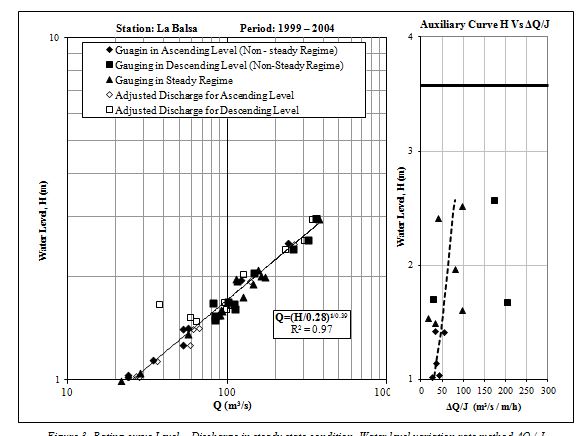
Figure 3 Rating curve Level - Discharge in steady state condition. Water level variation rate method ΔQ / J
| Time | H (m) | J (m/h) | (ΔQ/J) aj (m 3 /s/mh) | ∆Q= ∆Q/J*J (m 3 /s) | Q r (m 3 /s) | Q c (m 3 /s) |
|---|---|---|---|---|---|---|
| 06:00 | 2.20 | 0.23 | 70.00 | 15.75 | 189.23 | 204.98 |
| 07:00 | 2.52 | 0.32 | 78.00 | 24.96 | 268.34 | 293.30 |
| 08:00 | 2.84 | 0.32 | 103.00 | 32.96 | 364.94 | 397.90 |
| 10:00 | 3.05 | 0.11 | 124.00 | 13.02 | 438.44 | 451.46 |
| 10:20 | 2.91 | -0.42 | 118.00 | -49.56 | 387.96 | 3384 |
| 10:40 | 2.77 | -0.43 | 96.00 | -40.80 | 341.20 | 300.40 |
| 11:20 | 2.48 | -0.43 | 77.50 | -32.94 | 258.42 | 225.48 |
| 12:00 | 2.20 | -0.43 | 69.00 | -29.33 | 189.23 | 159.91 |
| 14:00 | 2.06 | -0.07 | 65.50 | -4.59 | 159.79 | 155.21 |
| 16:00 | 2.04 | -0.01 | 65.00 | -0.65 | 155.83 | 155.18 |
| 18:00 | 2.03 | -0.01 | 64.50 | -0.32 | 153.88 | 153.55 |
4. Conclusions
An important first step to obtain the rating curve in a station of a river is the analysis of the available information for the selection of the gauging data to be included in the procedure and, especially, the evaluation of the dynamics of the river to establish the type of dominant regime and the characteristics of the stretch and the natural conditions (discharge of a tributary, for example) and artificial conditions (a reservoir, a derivation, etc.) that may affect the Stage - Discharge relationship in the station.
The analysis of the variation of parameters, such as the hydraulic factor and the discharge as a function of the water level, the levels of the bed, the rates of variation of the water levels and the gradient of the free surface of water during the gauging, allows defining the characteristics of the gauging section, the type of the Stage - Discharge relationship and the procedures more appropriated to determine it. It also helps to establish the validity time of the curve.
To determine the simple rating curve in the La Balsa station, the logarithmic method was implemented because it allows identifying the type or types of control (section or channel) that determine the Stage - Discharge relationship and, therefore, extrapolate with less uncertainty the rating curve; in addition, it is easier to establish if there are changes in the type of control and, therefore, to determine with better precision the shape, curvature and tendency of the rating curve, for the different ranges of levels and in the transitions between two controls.
The operation of the Salvajina reservoir generates a dynamics of variation of water levels, depths, gradients, discharges and other parameters, which is reflected with greater intensity in the stations closest to the reservoir. This dynamic generates a complex relationship between stages and discharges (hysteresis phenomenon or process), and because of this the relationship presents a loop, indicating that for a given flood, in the same water level two different discharges occur (a higher discharge when the water level rises and a lower discharge when the water level decreases. Due to this, the Stage - Discharge relationship is complex and is conformed by the H-Q curve and an auxiliary curve that considers the different aspects that can affect it.
To find the complex rating curve in the La Balsa station (non-steady flow regime), the storage method per unit of variation rate in the levels (ΔQ/J) was implemented. This method shows significant differences in the discharges, when they are compared with those calculated using a simple rating curve (corresponding to steady regime). An example of application for the moderate flood of January 01 of 1999 shows differences of up to 19% between the discharges calculated through the two rating curves (steady and non-steady regimes).
Considering that the number of available gaugings in non-steady regime in the La Balsa station is limited, it is recommended to carry out additional gaugings both during the ascent and the descent of the water level, in order to characterize with greater detail the hysteresis phenomenon in the river and, therefore, define more accurately the auxiliary curve H vs. ΔQ/J.

