Estimation of the CO2 flux index in the San Andrés Island using fuzzy logic

Popayán, Juan G.; Becerra, Dorance; Zúñiga, Orlando; Popayán, Juan G.; Becerra, Dorance; Zúñiga, Orlando

doi:10.25100/iyc.v23i2.9700

Services on Demand

Journal

Article

Indicators

Cited by SciELO
Access statistics

Ingeniería y competitividad

Print version ISSN 0123-3033On-line version ISSN 2027-8284

Ing. compet. vol.23 no.2 Cali July/Dec. 2021 Epub May 18, 2021

https://doi.org/10.25100/iyc.v23i2.9700

Artículo

Estimation of the CO₂ flux index in the San Andrés Island using fuzzy logic

Estimación del índice de flujo de CO₂ en la isla de San Andrés mediante lógica difusa

Juan G. Popayán¹
http://orcid.org/0000-0001-7110-3371

Dorance Becerra²
http://orcid.org/0000-0001-8556-9914

Orlando Zúñiga¹
http://orcid.org/0000-0003-4434-8597

^¹Universidad del Valle, Departamento de Física, Cali, Colombia. Correo electrónico: juan.popayan@correounivalle.edu.co, orlando.zuniga@correounivalle.edu.co.

^²Universidad Francisco de Paula Santander, Departamento de Ciencias del Medio Ambiente, San José de Cúcuta, Colombia. Correo electrónico: dorancebm@ufps.edu.co.

Abstract

When applying fuzzy inference systems through the software to Spatial data processing for decision making (GeoFis) to a coral complex database of the island of San Andres, a CO₂ flux index was estimated that allows us to know the effect of the flux on the sea and the influence of the variables involved. It was found that six of the studied areas had a state of acidification of the sea due to CO₂, while all other areas had a slight incorporation of the gas. Likewise, it was evident that variables that have a significant influence on the incorporation of CO₂ into the marine environment are the sea surface temperature and the chemical nature of this gas, according to the component analysis. Therefore, the fuzzy methods for the determination of acidification of coral ecosystems, allows establishing an approachment effects from the gradual incorporation of CO₂ that would have into the marine environment, in addition to providing excellent advantages in terms of its determination based on satellite information.

Keywords: Acidification; CO2 flux; Fuzzy logic; GeoFIS

Resumen

Al aplicar sistemas de inferencia difusos a través del software de procesamiento de datos espaciales para la toma de decisiones (GeoFis) en una base de datos de complejo coralino de la isla de San Andrés se estimó un índice de flujo de CO₂ que permite conocer el efecto del flujo sobre mar y la influencia de las variables involucradas. Se encontró que seis de las zonas estudiadas tenían un estado de acidificación del mar por cuenta del CO₂, mientras todas las demás zonas tenían una leve incorporación del gas. Así mismo, se pudo evidenciar que las variables que poseen influencia significativa sobre la incorporación de CO₂ al medio marino son la temperatura superficial del mar y la naturaleza química de este gas, según el análisis de componentes. Por lo cual, los métodos difusos para la determinación de acidificación de los ecosistemas coralinos, permite establecer una aproximación a los efectos de la incorporación gradual de CO₂ que tendría en el medio marino, además de brindar excelentes ventajas en cuanto a su determinación a partir de información satelital.

Palabras clave: Acidificación; Flujo de CO2; GeoFIS; Lógica difusa

1. Introduction

Anthropogenic activities generate atmospheric emissions that increase as the population grows, these cause notable effects attributed especially to CO₂, which is derived from the burning of fossil fuels. Among the most relevant effects are global warming, climate change and damage to the biosphere, which are key issues today, since it causes multiple negative impacts according to Claesson & Nycander ¹, Lefevre ², and Koçak, Ulucak, & Ulucak ³.

Among the characteristics that make CO₂ creditor the most representative of the greenhouse gases that accelerate global warming, are long periods of permanence in the atmosphere for up to centuries, where about 46% of total emissions remain in the atmosphere, the high capacity to retain heat, in short, the large amounts emitted by human activities on a daily basis ⁴^,⁵. Thus, it has been shown that the adverse effects of this compound come to suffer from marine ecosystems ⁶^,⁷.

In effect, the oceans receive high amounts of CO2, of approximately 30% of the total emitted ⁴, this is possible due to the relationship between the water surface and the atmosphere where there is an exchange of gases ⁸. Therefore, consequences are generated in the marine environment due to the acidification of the oceans, particularly in coral reefs, which are vulnerable to these changes, which causes the availability of the necessary minerals that make up their skeletons (aragonite) and that carbonate ions are decreased, which produces a reduction in their calcification, which can cause the net loss of these strategic ecosystems, along with their ecosystem services ⁹^,¹⁰.

In this sense, in Colombia there is little scientific knowledge about the effects of climate change on its marine and coastal areas, which makes it impossible to structure national policies for the conservation of marine ecosystems, so it is necessary to establish indices that allow to know the state of the country's maritime sector.

Therefore, this article aims to establish a CO₂ flux index for the coral complex system of San Andrés Islas using inference systems through the GeoFIS tool, that is, this place is part of a conservation area, the largest declared Seafluxer Biosphere Reserve, where the diversity of marine ecosystems stands out, among the most important being coral reefs ¹¹.

2. Methodology

2.1. Place of study

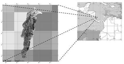
San Andrés islands is an archipelago that belongs to Colombia located in the southwest of the Caribbean (12-16 degrees latitude N. and 78-82 degrees latitude W.), declared by UNESCO as a Biosphere Reserve in 2001 under the administration of the Corporation for the Sustainable Development of San Andrés, Vieja Providencia and Santa Catalina, CORALINA ¹². In particular, the island of San Andrés is the largest with approximately 25 km² of emerging area, located about 290 km off the coast of Nicaragua (Central America) and 480 km off the coast of Cartagena (Colombia) ¹³, is characterized by being one of the main tourist attractions in the country, which has a wide diversity of marine fish and important ecosystems such as coral reefs, prairie beds, sandy coasts and mangroves ¹²^-¹⁴. The study area is shown in Figure 1.

Figure 1 San Andrés Island

2.2. Estimation of the CO₂ flux index

The determination of the CO₂ flux index requires defining the dependency functions that describe the behavior of each of the input variables in the fuzzy model, which can be obtained through specialized scientific literature, which helps to establish each variable, the function of relevance and function parameters.

Once the database is normalized, two files are created in comma-separated values (.csv) format for the aggregate variables of the transfer constant k or also CO₂ flow constant (made up of wind speed and sea surface temperature) and the partial pressure differential (ΔP) of CO₂ both in seawater and in the atmosphere.

For which, a partition is generated at 75% of the data for k and ΔP, a FIS without rules is generated and finally the performance of each sample is estimated. In this way determine the FIS rules to proceed to induce the rules through supervised learning type OLS. This procedure was repeated with each of the learning files, where it established the performance of each one by comparing the indices pi, RMSE, MAE, coverage, and maximum error.

Subsequently, the normalized database is loaded again to GeoFIS, with the corresponding coordinate system for Colombia (WGS 84 zone 18N), and then proceed to perform a data merge, where the membership functions that describe the behavior are defined. of each of the input variables in the fuzzy model.

On the other hand, for the determination of the CO₂ flux index, the Weighted Arithmetic Mean (WAM) operator is used, by means of the induced weights of the autonomous learning of the database, in this way to obtain the fusion of data for the calculation of the CO₂ flux indicator.

2.3. Performance criteria considered

Coverage ratio: Data rows are labeled as active or inactive for a given rule base. A row is active if its maximum match degree in all rules is greater than a defined threshold.
Following this definition, a coverage index value is calculated, which is a quality index complementary to classical precision.
Performance indices: Next, the error rate only considers the number of active elements defined above. For regression cases, the performance index available in FisPro (Fuzzy Inference System Professional) is based on the root mean square error (RMSE), Eq. 1:

RMSE=1A∑i=1Ay^-y12 (1)

Where y^1 is the inferred value (Eq. 2).

MAE= 1A∑i=1Ay^1-yi (2)

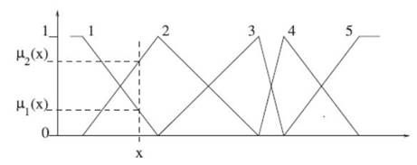
Linguistic Variable and Fuzzy Partitioning: Variable partitioning is the first step in FIS design. The conditions necessary for fuzzy partitions to be interpretable. The main points are distinction, a justifiable number of fuzzy sets, normalization, overlap and sufficient coverage: each data point, x, should belong significantly (l (x)> at least one fuzzy set is called the coverage level).

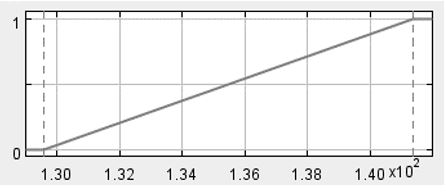
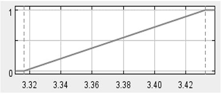
In this way, the linguistic rules can be interpreted as overlaps between functions, as shown in Figure 2:

Figure 2 Overlapping functions. Adapted from Guillaume & Charnomordic ¹⁵.

Induction of rules: FIS learning involves adjusting many parameters, so in this case it is feasible to consider only single output systems in the present study. Whatever its complexity and origin (fuzzy grouping, statistical methods, machine learning or ad hoc data-based designed specifically for fast learning of fuzzy rules). Once the input fuzzy partitions have been defined, we proceed to generate the complete set of rules corresponding to all combinations of fuzzy sets. For this case, due to the nature of the phenomenon and the available data, the Orthogonal Least Squares (OLS) method was used, which is a prototype-based learning method.

2.4. Data analysis

From three CO₂ flux scenarios, developed from a comparison of the fuzzy indicator with the linear method of estimating CO₂ flux, the results of each indicator can be placed within a range that allows us to know the effect of the flux, as shown in Table 1.

Table 1 CO₂ flux indicator ranges

Rank	Flux effects	References
0.0 - 0.3	Sea acidification due to CO₂.	¹⁶^-¹⁸
0.3 - 0.6	Slight incorporation of CO₂ into the sea.	¹⁸^-²⁰
0.6 - 1.0	CO₂ flux equilibrium	¹⁸^,²¹^,²²

2.5. Limiting factors

The principal component analysis is carried out with the purpose of establishing the variables or limiting factors of the CO₂ flux phenomenon. This procedure is executed through the Primer V6 software, available at https://www.primer-e.com/, which produces a graph showing the components that determine the behavior of the CO₂ flux.

3. Results y discussion

The relevance functions of the input variables in the fuzzy model and their characteristics are shown in Table 2.

Table 2 Membership functions for calculating the CO₂ flux index

Input variable	Function parameters	References
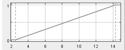
Wind speed	Semi trapezoidal sup. Bottom help: 2.5 lower Kernel:14.3	²³^-²⁵
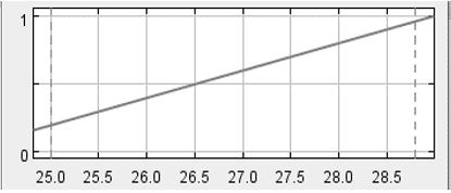
Sea Surface Temperature	Semi trapezoidal sup. Bottom help: 24 lower Kernel:29	²⁴^,²⁶
CO₂ Partial Pressure	Semi trapezoidal sup. Bottom help: 141.38 lower Kernel: 129.56	¹⁷^,¹⁹
CO₂ Partial Pressure	Semi trapezoidal sup. Bottom help: 343.26 lower Kernel:331.64	¹⁸^,²⁵^,²⁷

Table 2 summarizes the conceptual considerations regarding the relevance function and function parameters of each input variable included in the calculation of CO₂ flux.

Considering the information shown in Tables 3 and 4 about the performance and coverage indices for the data of k and ΔP, it was determined that the FIS (Fuzzy Inference System) rules to use correspond to sample 8 (simple 8) and sample 9 (simple 9) for each of these aggregate variables.

Table 3 Performance and coverage indices for the induction of OLS rules for k

	Sample 1	Sample 2	Sample 3	Sample 4	Sample 5	Sample 6	Sample 7	Sample 8	Sample 9
Pi	0.009	0.006	0.007	0.007	0.008	0.005	0.005	0.008	0.007
RMSE	0.05	0.034	0.034	0.038	0.042	0.027	0.029	0.046	0.039
MAE	0.036	0.027	0.029	0.031	0.035	0.02	0.023	0.038	0.031
Coverage	93	84	81	87	84	84	87	100	90
Maximum error	0.147	0.097	0.058	0.089	-0.0106	0.052	0.068	0.105	-0.11

Table 4 Performance and coverage indices for the induction of OLS rules for ΔP

	Sample 1	Sample 2	Sample 3	Sample 4	Sample 5	Sample 6	Sample 7	Sample 8	Sample 9
Pi	0.006	0.004	0.002	0.003	0.004	0.003	0.004	0.003	0.004
RMSE	0.031	0.022	0.011	0.019	0.019	0.019	0.024	0.014	0.02
MAE	0.02387	0.017	0.009	0.015	0.016	0.015	0.02	0.012	0.015
Coverage	87	93	90	93	87	90	93	90	90
Maximum error	-0.101	0.069	0.033	0.058	0.042	0.039	-0.045	0.034	0.066

Thus, the normalized database is loaded with the information again to GeoFIS, for the fusion of the data and subsequent use of the Weighted Arithmetic Mean (WAM) operator, obtaining the data of the fusion of data for the calculation of the CO₂ flux indicator shown in Table 5.

Table 5 Data fusion for the CO₂ flux indicator

Station	Flux _CO2 Index	K estimated	Temperature	Wind	Delta_P	PP_CO2_Water	PPT_CO2_Air
C1	0.49	0.4935	0.5400	0.8571	0.4898	0.4248	0.7304
C1a	0.47	0.4319	0.4000	0.8357	0.4983	0.5160	0.7168
C1b	0.50	0.5205	0.5400	0.8786	0.4851	0.4248	0.7036
C2	0.45	0.4638	0.6000	0.8214	0.4373	0.3876	0.4948
C2a	0.44	0.4581	0.7000	0.8214	0.4250	0.3272	0.4948
C2b	0.44	0.4581	0.7000	0.8214	0.4250	0.3272	0.4948
C3	0.40	0.3891	0.7800	0.7857	0.4155	0.2808	0.4948
C3 a	0.40	0.3777	0.8000	0.7857	0.4155	0.2808	0.4948
C3 b	0.43	0.4486	0.7000	0.7857	0.4155	0.2808	0.4948
Cove Seaside	0.42	0.3691	0.7400	0.0714	0.4607	0.3040	0.6904
Cove Seaside a	0.43	0.3840	0.8000	0.0714	0.4550	0.2696	0.6768
Cove Side b	0.42	0.3342	0.6000	0.0714	0.4765	0.3876	0.7036
Evans Point	0.43	0.3935	0.8800	0.1071	0.4515	0.2252	0.6904
Evans Point a	0.45	0.4521	0.9600	0.1071	0.4445	0.1824	0.6768
Evans Point b	0.43	0.4013	0.9000	0.1071	0.4519	0.2144	0.7036
Evans Point c	0.32	0.3630	0.8000	0.1786	0.2979	0.2696	0.2992
Genie Bay	0.32	0.3518	0.7400	0.1786	0.2930	0.3040	0.2860
Genie Bay a	0.32	0.3630	0.8000	0.1786	0.2979	0.2696	0.2992
Genie Bay b	0.39	0.2897	0.5000	0.3557	0.4612	0.4504	0.5340
German Point	0.31	0.3402	0.6600	0.1429	0.2975	0.3512	0.2992
German Point a	0.33	0.3687	0.8000	0.1429	0.3034	0.2696	0.3120
German point b	0.30	0.3123	0.6000	0.1429	0.2936	0.3876	0.2992
Low Bight	0.34	0.1783	0.4600	0.2143	0.4438	0.4764	0.4816
Low Bight a	0.37	0.2805	0.6000	0.2143	0.4305	0.3876	0.4868
Low Bight b	0.33	0.1783	0.4600	0.2143	0.4348	0.4764	0.4712
Low Bight c	0.33	0.1337	0.2000	0.2143	0.4653	0.6552	0.4816
Old Point	0.35	0.1783	0.3000	0.2143	0.4622	0.5840	0.4868
Old Point a	0.33	0.1337	0.2000	0.2143	0.4561	0.6552	0.4712
Old Point b	0.26	0.1373	0.2800	0.4286	0.3483	0.5984	0.3380
Pleasant Point	0.24	0.0874	0.3600	0.4286	0.3351	0.5428	0.3432
Pleasant Point a	0.26	0.1373	0.2800	0.4286	0.3442	0.5980	0.3328
Pleasant Point b	0.28	0.2646	0.6000	0.2500	0.2936	0.3876	0.2992
San Andres Bay	0.27	0.2295	0.5600	0.2500	0.3009	0.4124	0.3120
San Andres Bay a	0.29	0.3043	0.6600	0.2500	0.2880	0.3512	0.2860
San Andres Bay b	0.27	0.2170	0.6600	0.4643	0.2975	0.3512	0.2992
Sound Bay	0.22	0.1540	0.6000	0.4643	0.2681	0.3876	0.2656
Sound Bay a	0.24	0.1540	0.6000	0.4643	0.2976	0.3876	0.3044
Sound Bay b	0.22	0.0910	0.5400	0.4643	0.2996	0.4248	0.3120
South End	0.40	0.3342	0.6000	0.0714	0.4470	0.3876	0.5212
South End a	0.40	0.3254	0.5600	0.0571	0.4543	0.4124	0.5340
South End b	0.44	0.4320	0.8600	0.5000	0.4527	0.2360	0.6904
Sukey Bay	0.44	0.4320	0.8600	0.5000	0.4527	0.2360	0.6904
Sukey Bay a	0.42	0.3600	0.8000	0.5000	0.4581	0.2696	0.7036
Sukey Bay b	0.40	0.3120	0.7600	0.5000	0.4584	0.2924	0.6824

From the analysis presented as a similarity matrix in Table 6, the principal components analysis is performed, the result of which is shown in Figure 3.

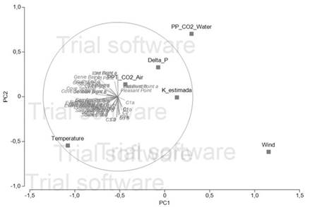
Figure 3 Principal component analysis for the CO₂ flux indicator on San Andrés Island. Source from: Author, 2020

According to the vector distribution of the variables that make up the CO₂ flux phenomenon in the different study areas on the San Andrés Island, it can be inferred that the CO₂ partial pressure and the wind speed do not condition the flux behavior in the marine environment, at least for the areas and at the time of study.

Table 6 Triangular matrix of similarity according to the Euclidean distance.

Samples
	K_estimated	Temperature	Wind	Delta_P	PP_CO₂_Water	PPT_CO₂_Air
K_estimada
Temperature	1.6515
Wind	1.5543	2.2521
Delta_P	0.88599	1.3934	1.5708
PP_CO₂_Water	1.3359	1.8632	1.6119	0.74628
PPT_CO₂_Air	1.1797	1.1839	1.8198	0.58104	1.2248

On the other hand, the CO₂ transfer coefficient, closely related to the sea surface temperature and the chemical nature of this gas, have a significant influence on the incorporation of this gas into the marine environment, these two variables being the flux limiting factors. CO₂ for this case study.

4. Conclusions

The application of fuzzy methods to determine the acidification of coral ecosystems allows establishing an approximation of the effects that the gradual incorporation of CO₂ would have into the marine environment, in addition to offering excellent advantages in terms of its determination based on reliable satellite information and easy access.

6. References

1. Claesson J, Nycander J. Combined effect of global warming and increased CO2 -concentration on vegetation growth in water-limited conditions. Ecological Modelling. 2013; 256: 23-30. doi: 10.1016/j.ecolmodel.2013.02.007. [ Links ]

2. Lefevre S. Are global warming and ocean acidification conspiring against marine ectotherms? A meta-analysis of the respiratory effects of elevated temperature, high CO2 and their interaction. Conservation Physiology. 2016; 4: cow009. doi: 10.1093/conphys/cow009. [ Links ]

3. Koçak E, Ulucak R, Ulucak ZS. The impact of tourism developments on CO2 emissions: An advanced panel data estimation. Tourism Management Perspectives. 2020;33(2019):100611. doi: 10.1016/j.tmp.2019.100611 [ Links ]

4. Intergovernmental Panel on Climate Change. Carbon and Other Biogeochemical Cycles. In: Cambridge University Press, editor. Climate Change 2013 - The Physical Science Basis: Working Group I Contribution to the Fifth Assessment Report of the Intergovernmental Panel on Climate Change. Cambridge: Cambridge University Press; 2014. p. 465-570. doi: 10.1017/CBO9781107415324.015. [ Links ]

5. MacDougall AH, Friedlingstein P. The Origin and Limits of the Near Proportionality between Climate Warming and Cumulative CO2 Emissions. Journal of Climate.2015;(2810):4217-4230. doi: 10.1175/jcli-d-14-00036.1. [ Links ]

6. Rau GH, McLeod EL, Hoegh-Guldberg O. The need for new ocean conservation strategies in a high-carbon dioxide world. Nature Climate Change. 2012;(210):720-724. doi: 10.1038/nclimate1555 [ Links ]

7. Szulejko JE, Kumar P, Deep A, Kim KH. Global warming projections to 2100 using simple CO2 greenhouse gas modeling and comments on CO2 climate sensitivity factor. Atmospheric Pollution Research. 2017;(81):136-140. doi: 10.1016/j.apr.2016.08.002. [ Links ]

8. Wong CS, Christian JR, Wong E, Page J, Xie L, et al. Carbon dioxide in surface seawater of the eastern North Pacific Ocean Line P., 1973-2005. Deep-Sea Research Part I: Oceanographic Research Papers. 2010; (575):687-695. doi: 10.1016/j.dsr.2010.02.003. [ Links ]

9. Tambutté E, Venn AA, Holcomb M., Segonds N, Techer N. et al. Morphological plasticity of the coral skeleton under CO2-driven seawater acidification. Nature Communications. 2015;6:7368. doi: 10.1038/ncomms8368. [ Links ]

10. Albright R, Takeshita Y, Koweek DA, Ninokawa A, Wolfe K. et al. Carbon dioxide addition to coral reef waters suppresses net community calcification. Nature. 2018; 555 (7697): 516-519. doi: 10.1038/nature25968. [ Links ]

11. Taylor E, Baine M, Killmer A, Howard M. Seafluxer marine protected area: Governance for sustainable development. Marine Policy. 2013;41:57-64. doi: 10.1016/j.marpol.2012.12.023. [ Links ]

12. Gavio B, Palmer-Cantillo S, Mancera JE. Historical analysis 2000-2005. of the coastal water quality in San Andrés Island, SeaFluxer Biosphere Reserve, Caribbean Colombia. Marine Pollution Bulletin. 2010; (607):1018-1030. doi: 10.1016/j.marpolbul.2010.01.025. [ Links ]

13. Albis-Salas MR, Gavio B. Notes on marine algae in the International Biosphere Reserve Seaflower, Caribbean Colombian I: new records of macroalgal epiphytes on the seagrass Thalassia testudinum. Botanica Marina. 2011; (546): 537-543. doi: 10.1515/BOT.2011.069. [ Links ]

14. Castaño-Isaza J, Newball R, Roach B, Lau WWY. Valuing beaches to develop payment for ecosystem services schemes in Colombia's Seafluxer marine protected area. Ecosystem Services. 2015;11:22-31. doi: 10.1016/j.ecoser.2014.10.003. [ Links ]

15. Guillaume S, Charnomordic B. Learning interpretable fuzzy inference systems with FisPro. Information Sciences. 2011; (18120):4409-4427. doi: 10.1016/j.ins.2011.03.025. [ Links ]

16. Dong F, Zhu X, Qian W, Wang P, Wang J. Combined effects of CO2-driven ocean acidification and Cd stress in the marine environment: Enhanced tolerance of Phaeodactylum tricornutum to Cd exposure. Marine Pollution Bulletin. 2020;150 (2019): 110594. doi: 10.1016/j.marpolbul.2019.110594. [ Links ]

17. Orselli IBM, Goyet C, Kerr R, de Azevedo JLL, Araujo M. et al. The effect of Agulhas eddies on absorption and transport of anthropogenic carbon in the South Atlantic Ocean. Climate. 2019;(76): 84. doi: 10.3390/CLI7060084. [ Links ]

18. Padin XA, Castro CG, Ríos AF, Pérez FF. Oceanic CO2 uptake and biogeochemical variability during the formation of the Eastern North Atlantic Central water under two contrasting NAO scenarios. Journal of Marine Systems. 2011; (843-4): 96-105. doi: 10.1016/j.jmarsys.2010.10.002. [ Links ]

19. D'Ortenzio F, Antoine D, Marullo S. Satellite-driven modeling of the upper ocean mixed layer and air-sea CO2 flux in the Mediterranean Sea. Deep-Sea Research Part I: Oceanographic Research Papers. 2008;(554):405-434. doi: 10.1016/j.dsr.2007.12.008. [ Links ]

20. Else BGT, Yackel JJ, Papakyriakou TN. Application of satellite remote sensing techniques for estimating air-sea CO2 fluxes in Hudson Bay, Canada during the ice-free season. Remote Sensing of Environment. 2008; (1129):3550-3562. doi: 10.1016/j.rse.2008.04.013. [ Links ]

21. Hattam C, Atkins JP, Beaumont N, Börger T, Böhnke-Henrichs A, et al. Marine ecosystem services: Linking indicators to their classification. Ecological Indicators. 2015; 49: 61-75. doi: 10.1016/j.ecolind.2014.09.026. [ Links ]

22. Takahashi T, Sutherland SC, Chipman DW, Goddard JG, Ho C. et al. Climatological distributions of pH, pCO2, total CO2, alkalinity, and CaCO3 saturation in the global surface ocean, and temporal changes at selected locations. Marine Chemistry. 2014; 164: 95-125. doi: 10.1016/j.marchem.2014.06.004. [ Links ]

23. Soloviev A, Donelan M, Graber H, Haus B, Schlüssel P. An approach to estimation of near-surface turbulence and CO2 transfer velocity from remote sensing data. Journal of Marine Systems. 2007; (661-4): 182-194. doi: 10.1016/j.jmarsys.2006.03.023. [ Links ]

24. Woods S, Minnett PJ, Gentemann CL, Bogucki D. Influence of the oceanic cool skin layer on global air-sea CO2 flux estimates. Remote Sensing of Environment. 2014;145:15-24. doi: 10.1016/j.rse.2013.11.023. [ Links ]

25. Yasunaka S, Murata A, Watanabe E, Chierici M, Fransson A. et al. Mapping of the air-sea CO2 flux in the Arctic Ocean and its adjacent seas: Basin-wide distribution and seasonal to interannual variability. Polar Science. 2016; (103): 323-334. doi: 10.1016/j.polar.2016.03.006. [ Links ]

26. Chien H, Zhong YZ, Yang KH, Cheng HY. Diurnal variability of CO2 flux at coastal zone of Taiwan based on eddy covariance observation. Continental Shelf Research. 2018; (162): 27-38. doi: 10.1016/j.csr.2018.04.006. [ Links ]

27. Wanninkhof R, Barbero L, Byrne R, Cai WJ, Huang WJ. et al. Ocean acidification along the Gulf Coast and East Coast of the USA. Continental Shelf Research. 2015; 98: 54-71. doi: 10.1016/j.csr.2015.02.008. [ Links ]

Notes:

5. Funding Statement The author(s) received no specific funding for this work.

Como citar: Popayán JG, Becerra D, Zúñiga O. Estimación del índice de flujo de CO₂ en la isla San Andrés mediante lógica difusa. INGENIERÍA Y COMPETITIVIDAD. 2021;23(2):e2039700. https://doi.org/10.25100/iyc.v23i2.9700

Received: May 13, 2020; Accepted: March 07, 2021

This is an open-access article distributed under the terms of the Creative Commons Attribution License