WHICH COST OF DEBT SHOULD BE USED IN FORECASTING CASH FLOWS?*

IGNACIO VÉLEZ–PAREJA

Master of Science in Industrial Engineering, University of Missouri, United States. Associated Professor, Universidad Tecnológica de Bolívar, Colombia. Corresponding address: Calle del Bouquet #25-92, Manga, Cartagena, Colombia. nachovelez@gmail.com

Fecha de recepción: 26-03-2008 Fecha de corrección: 13-03-2009 Fecha de aceptación: 20-04-2009

* This research was financed by the Universidad Tecnológica de Bolívar, Cartagena, Colombia.

ABSTRACT

Frequently, analysts and teachers use the capitalized rate of interest for the cost of debt when forecasting and discounting cash flows. Others estimate the interest payments when forecasting annual financial statements or cash flows based on the average of debt calculated with the beginning and ending balance. Others use the end of year convention that calculates the yearly interest multiplying the beginning balance times its contractual cost. The use of one or other methods is critical for the definition of the tax savings. These approaches are illustrated with examples and the differences in using them. A simple proposal to solve the problem is presented.

KEYWORDS

Cost of debt, forecasting financial statements, seasonality.

JEL Classification: G30, G31, G32

RESUMEN

¿Qué costo de deuda debe ser usado para pronosticar los flujos de caja?

Con frecuencia analistas y profesores utilizan la tasa de interés efectiva para estimar el costo de la deuda para pronosticar y descontar los flujos de caja. Otros estiman los pagos de interés basados en el promedio de la deuda calculado con el saldo inicial y final. Otros más utilizan la convención de final de período y calculan el interés multiplicando el saldo inicial de la deuda por su costo contractual. El uso de uno u otro método es crítico para el cálculo de los ahorros en impuestos. Se ilustran estos enfoques con ejemplos y se muestran las diferencias al usarlos. Se presenta una propuesta simple para solucionar el problema.

PALABRAS CLAVE

Costo de la deuda, proyecciones de estados financieros, estacionalidad.

INTRODUCTION

Frequently analysts and teachers use the capitalized rate of interest for the cost of debt when forecasting and discounting cash flows and calculating the cost of capital (Benninga & Sarig, 1997; Berk & DeMarzo, 2009; Brealey & Myers, 2003; Copeland & Weston, 1988; Grinblatt & Titman, 2001; Ross, Westerfuekd y Jaffe, 1999). On the other hand, some authors (and analysts) estimate the interest payments when forecasting annual financial statements or cash flows based on the average of debt calculated with the beginning balance and the end of year balance (Benninga, 2006; Day, 2001; Tjia, 2004). This makes some sense because usually firms repay debt in a monthly or quarterly basis and calculating interest payments on an annual basis might not reflect reality, however, circularity will arise. Others use the end of year convention that calculates the yearly interest multiplying the beginning balance times the contractual cost of debt (Tham & Vélez-Pareja, 2004). Moreover, an example adapted from Vélez-Pareja (2006) is presented, where even calculation of interest when forecasting and interest liquidation period coincide with the same period of analysis and a distortion in the Kd, the cost of debt, is found.

The problem of these approaches is that they might not reflect the correct cost of debt and conceal the actual tax savings earned when valuing a cash flow with a discount rate that takes into account the tax shields (Tham & Vélez-Pareja, 2004; Vélez-Pareja & Benavides, 2006; Vélez-Pareja, Ibragimov y Tham, 2008). In this work the differences when using those approaches are shown and a simple proposal to solve the problem is shown.

The document is organized as follows: Section One presents four possible approaches to solve this situation. Section Two presents a simple example for quarterly and monthly interest charges and compares the differences among the four approaches. Section Three concludes.

1. FOUR POSSIBLE APPROACHES

This Section presents four possible approaches to estimate the interest expenses when forecasting financial statements: The first is the use of the capitalized interest rate; the second one is to average debt to calculate interest payments with the contractual cost of debt, Kd; the third procedure uses the sum of the actual interest payments in the year when the interest is liquidated in shorter periods than the one used to forecast; and finally, the last one uses of contractual cost of debt Kd and the end of year assumption where the interest charges are calculated with Kd and the initial debt balance. It is possible to find other versions that combine some of the four approaches described herein.

1.1. Use of capitalized interest rate

There is no firm that pays the capitalized interest rate. There is no bank that calculates the interest payments based on the capitalized interest rate. This is very important either for forecasting financial statement or discounting cash flows using the well known formulation for the Weighted Average Cost of Capital (WACC).

The capitalized interest rate is a mathematical construct. It is a fiction. One thing that sheds light over the inappropriateness of the practice is that it assumes that the firm can invest the borrowed amount at the same cost of debt. That is what is implicit in the well known formula for capitalizing interest:

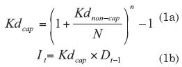
Where Kd_cap is the capitalized interest rate, Kd_non–cap is the non capitalized rate, I is the interest charge and N is the period of liquidation of interest.

1.2. Use of average debt to calculate interest payments

In this case the interest payment is calculated using the contractual cost of debt (Kd_non–cap) and the debt to calculate interest charges is the average between the beginning and end of year balance. This is:

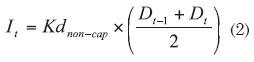
Where I_t is the interest payment, Kd_non–cap is the contractual cost of debt and D is the debt balance at the beginning and end of year (Benninga, 2006; Tjia, 2004).

This approach is a proxy that takes into account that the debt balance decreases if debt is repaid during the year, or increases if new debt is contracted.

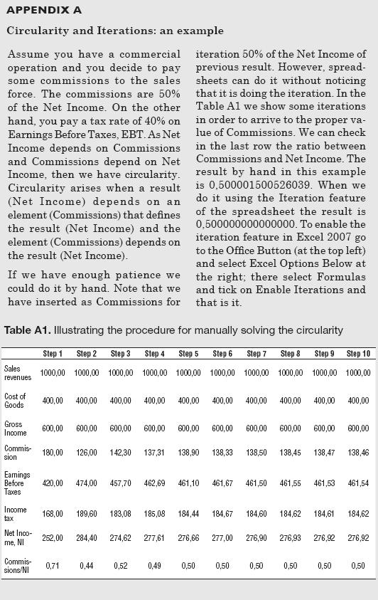
As we use debt in period t that depends on the interest payments of that year, circularity arises. See an example of circularity in Appendix A.

1.3. Use of the sum of the actual interest payments in the year

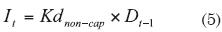
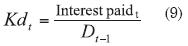
If the analyst knows that debt is paid during the year on a non yearly basis she should calculate the actual amount paid during the year. This actual amount paid should be the basis to calculate the actual cost of debt the firm pays if the forecasts are calculated on a yearly basis. This is to say that the annual cost of debt is:

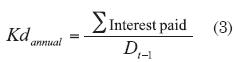
Kd_annual is the cost of debt on an annual basis, Interest paid is the interest charges based on the Kd_non–cap according to the capitalization period, and D_t–1 is the beginning balance debt. This approach is critical when discounting cash flows and using any of the multiple formulations for the WACC. The critical issues are the actual interest charges that the firm pays during the year and the tax savings (or tax shield), TS, the firm earns when the income tax is applied. It is well known that in absence of other sources of financial expenses, the TS is calculated as:

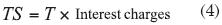
This means that for cash flow valuation purposes the two previous approaches (equations (1) and (2)) are wrong because they do not measure the actual interest charges and will distort the estimate for TS. The correct TS are earned on the interest actually paid by the firm. If calculation of periodical interest is based on periods shorter than a year (say, months, quarters, etc.) and the forecasting is based on years, then the TS should be calculated on the interest charges that result from a debt schedule constructed with the shorter periods.

1.4. Use of the contractual Kd and end of year assumption

With this approach the assumption is that there is not interest liquidation in shorter periods within the year, the calculation of interest charges is based on the beginning balance of debt and it occurs at the end of the year (Day, 2001; Tham & Vélez-Pareja, 2004). Obviously, usually there are principal payments during the year and this approach overestimates the interest paid.

In the next section an example to illustrate the under or overestimation is presented.

2. AN EXAMPLE WITH DIFFERENT APPROACHES

Assume a firm with an initial debt of 1.000, a contractual cost of debt, Kd of 12% per annum capitalized in four quarters and in twelve months. The debt schedule is calculated for monthly and quarterly payments. The payment of this initial debt decreases debt until it is fully repaid. This example will be used to evaluate the above mentioned approaches.

If the capitalized cost of debt is calculated for the two terms (four quarters and twelve months) then the cost of debt is 12,55% for the quarterly payments and 12,68% for the monthly payments.

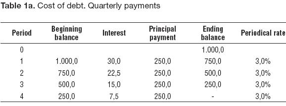
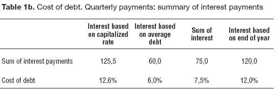
The debt schedule for quarter payments is as in Table 1a, from which the respective cost of debt based on the beginning of the year balance can be calculated (Table 1b). It is assumed that the charge and/or payment is done at the end of year.

In Table 2a the reader can see the same situation for monthly payments, when the respective cost of debt based on the beginning of the year balance can be calculated (Table 2b). It is assumed that the charge and/or payment are done at the end of year.

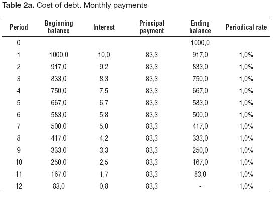
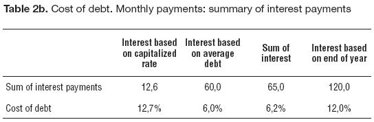
The actual interest paid (as can be seen in previous tables) is the sum of calculated interest. This is, 75 for quarters and 65 for months.

When the average of debt is used, the annual cost of debt is lower than the actual interest payments. When interest calculated with capitalized rate and end of year approaches is higher than the actual interest charges and the interest calculated with the average of debt approach is lower than the actual interest charges.

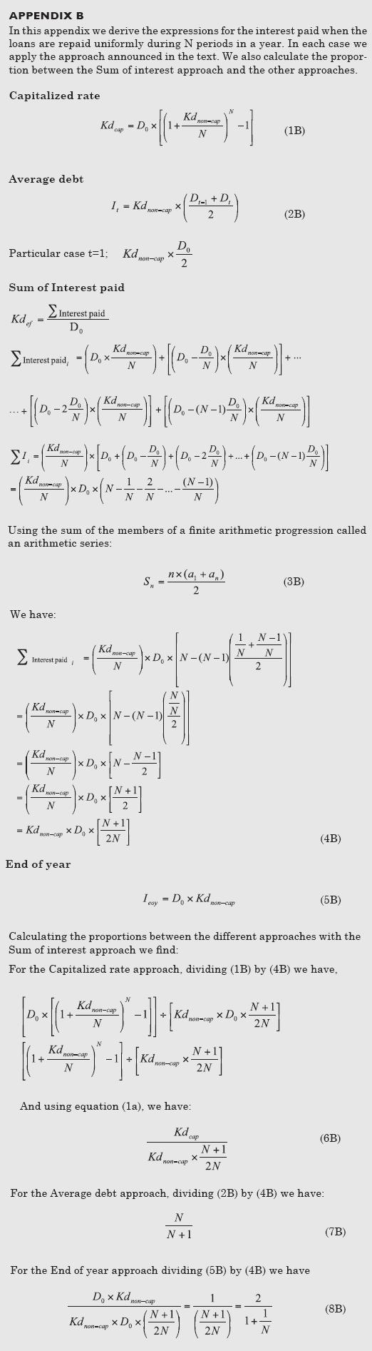
Appendix B shows the proportions between the different approaches with the actual calculated interest (sum of interest approach) for a decreasing to zero debt schedule for a year.

When the approach of capitalized interest rate is compared with the sum of interest charges the relation is:

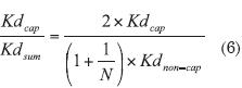
For N = 12 that value is 1,951154

For N = 4 that value is 1,6734508

In this case it can be seen that the capitalized cost of debt approach overestimates the cost of debt compared with the sum of interest charges. The greater the number of capitalization periods, N, the greater the overestimation with

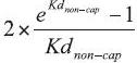
as an upper limit.

When the approachof end of year assumption is compared with the sum of interest charges the relation is:

For N = 12 that value is 1,846

For N = 4 that value is 1,6

In this case, the end of year approach overestimates the cost of debt compared with the sum of interest charges. The greater the number of capitalization periods, N, the greater the overestimation with 2 as an upper limit. This means that when N is too large, the end of year approach will double the sum of interest charges approach.

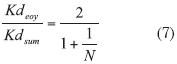
The proportion between averaging debts compared with the approach of sum of interest charged is:

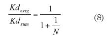
For N = 12 that value is 0,923

For N = 4 that value is 0,8

In this case, the average approach underestimates the cost of debt compared with the sum of interest charges. The greater the number of capitalization periods, N, the greater the overestimation with 1 as an upper limit. This means that when N is too large, the two approaches are equivalent.

Now the different approaches are compared for quarterly and monthly payments to examine the overestimation or underestimation of the cost of debt for different levels of contractual cost of debt, Kd. Table 3a shows the situation for quarterly payments.

For monthly payments the situation is as in Table 3b.

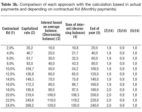
It is confirmed that the behavior of the approach based on average debt under estimates the interest charges and hence, the TS and the behavior of the capitalized rate and end of year calculation using the contractual cost of debt results in strong overestimation for the case of decreasing balance debt schedule. The higher the number of capitalization periods the higher the differences between end of year and end of year approaches with actual interest payments and the lower average debt approach with actual interest payments. This can be seen as well in equations (6), (7) and (8).

Even with annual payments with no liquidation in shorter periods one can find the problem of distortion of the Kd compared with the contractual borrowing rate. This is a typical problem found in real life by analysts and consultants. Firms have several loans, with different terms and cost of debt. In fact, the ideas developed in this work came from author’s consulting experience. This is illustrated with the following example.

Assume a firm with three loans: ten millions to be repaid in one year in only one payment with interest rate of 35% per annum; forty millions to be repaid in ten years, in constant payments, at an interest rate of 25% per annum; and forty millions repaid in five years with equal payments at 30% per annum.

The three debt schedules will be as follows:

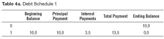
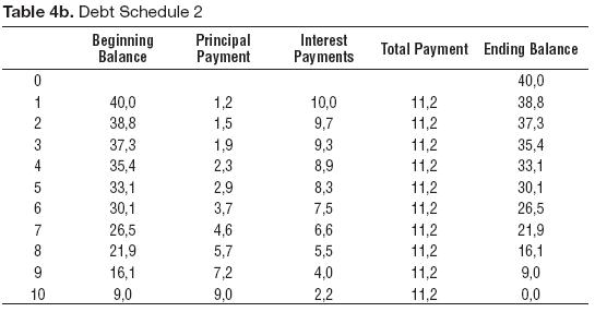
In Table 4a, the loan is repaid in one year and the cost of debt is 35%; while in Table 4b, it is presented the uniform payment for ten years and at a cost of debt of 25% per annum where the principal payment and the interest payment from total payment were disaggregated.

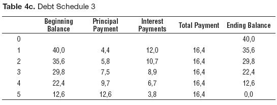
In Table 4c, the uniform payment for five years at a cost of debt of 30% per annum is presented, and as before, the principal payment and the interest payment from total payment has been disaggregated.

In Table 4d, the three debt schedules to see the total financing for the firm are shown.

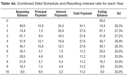
Last column, Kd, has been calculated as interest charges divided by the beginning balance. For instance, for year 1 we have 25,5/90,0 = 28,33%. Observe that the cost of debt varies from 25,0% up to 28,33% and it results from the combination of the three loans with different terms and interest rates. The calculation for the first year coincides with the average of the contractual cost of debt weighted by the debt balance in time 0. It is correct in that case but we cannot use that average for every year because the proportion does change and we have to take into account the debt balances for each year. Dividing the interest paid by the debt at the beginning of the year, takes into account the proper weights.

We can observe that a Kd based on a weighted average for the cost of debt with the initial debt balances or the Internal Rate of Return for the loans (27,37%) distort a reality that has to be taken into account: the cost of debt might (and usually does) change every period.¹ The amount of debt also changes as loans are repaid and/or the firm contracts other loans.

In short, the correct way to estimate the cost of debt when forecasting cash flows is:

Now the question is how to solve this problem, and which approach should be used. Very easy: none. With the use of spreadsheets it is possible to apply a general rule;² use a period consistent with the pattern of the debt schedule. Using the period of forecasting consistent with the pattern of repayment of debt has an additional advantage: the problem of monthly or quarterly seasonality is solved. It is not necessary to make approximations or to use algorithms to take into account that behavior.

However, if the analyst prefers to forecast on a yearly basis, she must add interest paid in shorter periods and estimate the cost of debt for cost of capital estimation purposes using (9).

The use of forecasting periods different from the year poses a problem that can be solved with careful modelling. Taxes are accrued during the current year and might be paid in different patterns. One of the most common ways to pay taxes is to pay total tax amount the following year or part in the current year and the rest in the following year. This means that it is necessary to know the rules for tax payment for the specific country or industry the analyst is dealing with.

3. CONCLUDING REMARKS

This document has shown the behavior of four approaches to determine what the cost of debt, Kd, will be when forecasting financial statements. The comparison has been made with the cost of debt, Kd, calculated as the actual interest charges divided by the initial debt balance. These four approaches are: a) the capitalized interest rate, b) the interest charges calculated on the basis of average debt (average of initial debt balance and end debt balance), c) Kd calculated as the sum of interest charges (defined for shorter periods (months or quarters), and d) the end of year model that assumes that the interest charges should be calculated using the contractual Kd and the initial debt balance.

The comparison has been made with approach c) because that approach is consistent with the tax savings (tax shields, TS) that are included in the valuation of cash flows when the Weighted Average Cost of Capital (WACC) is used as the discount rate; this is, TS are earned on the actual interest charged. That approach takes into account the correct amount of interest charges for defining the TS when constructing the discount rate (WACC).

The results from tables 3a and 3b and equations (6), (7) and (8) show that:

1. The capitalized interest cost of debt, Kd_cap, approach and the end of year approach strongly overestimate Kd and hence TS. See equations (6) and (7).
2. The cost of debt calculated based on the average debt systematically underestimates the contractual cost of debt and hence TS. See equation (8).

As a recommendation for forecasting it is suggested to coincide the period of forecasting with the period of calculation of interest charges. If not possible to forecast this way, calculate the cost of debt as financial expenses for the period divided by debt in the previous period. If the analyst needs to work with years she has to calculate the interest payments in shorter periods and add them up for the year, because this is the basis of the TS calculation.

FOOTNOTE

1. There might be several other reasons why the cost of debt varies, among others, the inflation rate.

2. The latest version of Excel MS Office (2007) has more than 16,000 columns (and more than one million lines) that allows for more than 44 years if forecast is done on a daily basis. We are sure that this is enough for any real life forecasting exercise.

BIBLIOGRAPHY

1. Benninga, S. (2006). Principles of Finance with Excel. London, UK: Oxford.        [ Links ]

2. Benninga, S., & Sarig, O. (1997). Corporate Finance. A Valuation Approach. New York, NY: McGraw- Hill.        [ Links ]

3. Berk, J., & DeMarzo, P. (2009). Corporate Finance: The Core. Boston, MA: Pearson Prentice-Hall.        [ Links ]

4. Brealey, R.A., & Myers, S.C. (2003). Principles of Corporate Finance (7th ed.). Boston, MA: McGraw-Hill/Irwin        [ Links ]

5. Copeland, T.E., & Weston, J.F. (1988). Financial Theory and Corporate Policy (3rd ed.). Reading, MA: Addison Wesley.        [ Links ]

6. Day, A. (2001). Mastering Financial Modelling. A Practitioner’s Guide to Applied Corporate Finance. London, UK: Prentice Hall.        [ Links ]

7. Grinblatt, M., & Titman, S. (2001). Financial Markets and Corporate Strategy (2nd ed.). Boston, MA: McGraw-Hill Irwin.        [ Links ]

8. Ross, S.A., Westerfield, R.W., & Jaffe, J. (1999). Corporate Finance (5th ed.). New York, NY: Irwin-McGraw-Hill.        [ Links ]

9. Tham, J., & Vélez-Pareja, I. (2004). Principles of Cashflow Valuation. An Integrated Market Value Approach. Boston, MA: Academic Press        [ Links ]

10. Tjia, J.S. (2004). Building Financial Models. A Guide to Creating and Interpreting Financial Statements. New York, NY: McGraw-Hill.        [ Links ]

11. Vélez-Pareja, I. (2006). Decisiones de Inversión. Para la valoración financiera de proyectos y empresas (5th ed.). Bogotá, Colombia: Universidad Javeriana.        [ Links ]

12. Vélez-Pareja, I., & Benavides, J. (2006). There Exists Circularity between WACC and Value? Another Solution. Estudios Gerenciales, 98, 13-23.        [ Links ]

13. Vélez-Pareja, I., Ibragimov, R., & Tham, J. (2008). Constant Leverage and Constant Cost of Capital: A Common Knowledge Half-Truth. Estudios Gerenciales, 24(107), 13- 34.        [ Links ]