POTENTIAL DIVIDENDS AND ACTUAL CASH FLOWS. A REGIONAL LATIN AMERICAN ANALYSIS¹

IGNACIO VÉLEZ-PAREJA*¹, MARIANO GERMÁN MERLO², DAVID ANDRÉS LONDOÑO BEDOYA³, JULIO ALEJANDRO SARMIENTO SABOGAL⁴

¹Master of Science en Industrial Engineering, University of Missouri, Estados Unidos. Profesor Asociado, Universidad Tecnológica de Bolívar, Colombia. Grupo de investigación Instituto de Estudios para el Desarrollo, IDE, Colombia. Dirigir correspondencia a: Universidad Tecnológica de Bolívar, Calle del Bouquet No 25-92, Manga, Cartagena, Colombia ivelez@unitecnologica.edu.co

²Máster en Finanzas, Universidad del CEMA, Argentina. Director Académico, Especialización en Análisis Financiero y Coordinador Académico del MBA mención Finanzas, Escuela de Negocios de la Universidad de Belgrano, Argentina. mariano.merlo@comunidad.ub.edu.ar

³PhD en Teoría Económica e Instituciones, Universitá degli Studi di Roma “Tor Vergata”, Italia. Profesor Investigador y Secretario Académico (e), Universidad Tecnológica de Bolívar, Colombia. Grupo de investigación Instituto de Estudios para el Desarrollo, IDE, Colombia. dlondono@unitecnologica.edu.co

⁴Especialista en Finanzas, Pontificia Universidad Javeriana, Colombia. Coordinador Académico Especialización en Gerencia Financiera, Pontificia Universidad Javeriana, Colombia. sarmien@javeriana.edu.co

* Autor para correspondencia.

Fecha de recepción: 08-06-2009 Fecha de corrección: 20-11-2009 Fecha de aceptación: 26-11-2009

ABSTRACT

We examine the value market assigns to components of the cash flow to equity including potential dividends. We study non financial publicly traded firms from five Latin American countries. The model includes four variables: market value of equity, dividends paid, change in equity investment and change in liquid assets (potential dividends) and are regressed with actual equity value as dependent variable. Tests applied give robust results. The main conclusions: Market assigns less than one dollar to a future dollar for any of the variables studied. Potential dividends destroy value. A dollar invested in liquid assets has a negative Net Present Value and it is not zero NPV investments. We confirm the agency costs of keeping undistributed cash flows.

KEYWORDS

Cash flow to equity, potential dividends, equity value.

JEL Classification: M41, G12, G31.

RESUMEN

Dividendos potenciales y flujos de caja: un análisis regional para América Latina

Se examina el valor que el mercado asigna a los componentes del flujo de caja del accionista, incluidos los dividendos potenciales. Se estudia empresas transadas de cinco países de América Latina. El modelo incluye cuatro variables: valor de mercado del patrimonio, los dividendos pagados, cambio en la inversión de patrimonio y cambio en activos líquidos (dividendos potenciales) y se regresaron con el valor de mercado del patrimonio como variable dependiente. Las pruebas estadísticas dan resultados sólidos. Conclusiones: El mercado asigna menos de 1 dólar a un dólar futuro para cualquiera de las variables. Los dividendos potenciales destruyen valor. Un dólar invertido en activos líquidos tiene un valor presente neto negativo. Confirmamos los costos de agencia de no distribuir los flujos de caja.

PALABRAS CLAVE

Flujo de caja del accionista, dividendos potenciales, valor del patrimonio.

RESUMO

Potenciais dividendos e fluxo de caixa efetivos: uma análise regional Latino Americana

Examinámos o valor que o mercado determina para componentes do fluxo de caixa, e para valoração do património, incluindo potenciais dividendos. Estudámos firmas não financeiras de capital aberto de cinco países Latino Americanos. O modelo inclui as quatro variáveis seguintes: valoração de patrimônio no mercado, dividendos pagos, mudança no investimento de patrimônio, e mudança em ativos disponíveis (potenciais dividendos). Foi realizada uma análise de regressão a essas variáveis usando valor de património real como uma variável dependente. Os testes efetuados produziram resultados fortes. As conclusões principais são as seguintes: o mercado determina menos de um dólar para um futuro dólar por qualquer das variáveis em revista. Potenciais dividendos destruem o valor. Um dólar investido em ativos disponíveis tem um Valor Líquido Presente negativo e não é investimento zero VPL. Nós confirmámos os custos da agência por manter fluxos de caixa retidos.

PALAVRAS-CHAVE

Fluxo de caixa para valoração, potenciais dividendos, valoração de patrimônio.

INTRODUCTION

We have examined the value that the market assigns to different components of the cash flow to equity including potential dividends. The theoretical and basic methodology of this work was developed by Vélez- Pareja and Magni (2009).

Our study is about non financial publicly traded firms in five Latin American countries: Argentina, Brazil, Chile, Mexico and Peru, during the period 1991-2007. The model includes the following variables: market value of equity, dividends paid, change in equity investment and change in liquid assets (potential dividends). These variables are regressed with actual equity value (time t) as a dependent variable and the other variables as independent variables (including equity value) for a next period (time t+1). Tests applied have given solid results.

We are concerned with the value the market assigns to the components of the Cash Flow to Equity, CFE, in particular to the change in liquid assets. Common practice assumes it is distributed among shareholders although in reality or in the typical financial model used to derive the cash flows, it is not because it is listed in the balance sheet.

There are three main conclusions in this work: in first place, the market assigns less than one dollar today to a future dollar for any of the variables studied as expected. Secondly, in particular, we found that potential dividends (changes in liquid assets) destroy value. In other words, the value of a dollar today in liquid assets in t+1, is negative. Third, we have found that, contrary to common knowledge and assumptions, a dollar invested in liquid assets has a negative Net Present Value (NPV) and they are not zero NPV investments. These findings confirm the agency costs of the problem when undistributed cash flows are kept. It also confirms that liquid assets should not be included in the cash flows while being listed in the balance sheet as current practice does.

According to Damodaran (2008, p. 106): “In the strictest sense, the only cash flow that an investor will receive from an equity investment in a publicly traded firm is the dividend that will be paid on the stock.” We adhere to this definition. Usually practice and textbooks consider the working capital for cash flow calculation, excluding liquid assets. The net effect of this is the increase of the cash flows by a sum that is listed in the balance sheet; hence it is not effectively received by the shareholder. This amount is the increase in liquid assets. In section one we show how this occurs. As a result, equity and firm value are overvalued.

On the other hand, when we analyze the change in liquid assets, we find that it is part of the cash flow generated by the investment in liquid assets; hence, when included in the cash flows, they are discounted to present value. This is part of the above overvalued value. However, the same common practice assumes that liquid assets are zero NPV investments. For this reason, the actual book value of liquid assets is added to the present value of the cash flows.

Empirical evidence suggests that we should abolish the practice of excluding from the working capital the liquid assets and adding the book value of liquid assets under the assumption that they are zero NPV investments. The only relevant cash flow is what effectively an investor receives from the equity investment: dividends and stock repurchases.

The article is organized as follows: in section one we define the problem and present a review of the current literature. In section two we describe in detail the theoretical model and propose the hypotheses. In section three we describe the data analyzed. In section four we analyze the data using ordinary linear regression OLS. In Section Five we present our conclusions.

1. BACKGROUND

In this Section we define the problem and present a literature review. What we find as a problem is an overvaluation of firm and equity value.

1.1. The problem

It is a well spread practice among authors, teachers and practitioners to include undistributed dividends as part of the Cash Flow to Equity (CFE) (and hence in the Free Cash Flow, FCF).

This happens when in the process of calculating working capital only non cash items are included. Working Capital (WC), is defined as the difference between current assets (cash (C) + short-term investments (STI) + accounts receivable (AR) + inventories (Inv)) - current liabilities (accounts payable (AP)):

The usual procedure to estimate the CFE in an indirect way departing from the income statement is the following:

Where CFE is cash flow to equity; NI is net income; ΔNFA_t+1 is investment in fixed assets ( ΔNFA_t+1 = NFA_t+1 – NFA_t = investment in Fixed Assets_t+1 –Depreciation _t+1; and represents the so-called Net Capital Expenditure); ΔWC is change in working capital; and ΔD is change in book value of debt.

By contrast, a frequent definition in textbooks turns out to be:²

With WC^nc being noncash (operating) working capital:

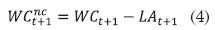
Where LA is liquid assets (C+STI), so that ΔAR_t+1 + ΔInv_t+1 – ΔAP_t+1 = ΔWC^nc_t+1(see, for example, Benninga, 2006, p. 271, Damodaran, 1999, p. 128; Damodaran, 2006a, p. 79). In eq. (2) change in working capital is inclusive of undistributed potential dividends ΔLA_t+1, whereas in eq. (3) change in working capital excludes ΔLA_t+1. That is the reason why the term in parenthesis in eq. (2) is greater than the term in parenthesis in eq. (3). As a result, CFE is smaller than CFE*. The missing term ( LA) is the so called potential dividends. Potential dividends overvalue actual cash flows and, hence, firm value.³

In fact, the term potential dividends has been coined by Damodaran (2008, pp. 205-206) and accepted by other authors (Benninga, 2006; Benninga and Sarig, 1997; Brealey and Myers, 2003; Copeland et al.,⁴ 1990; Damodaran, 2006a, 2006b).

Another assumption usually made is that investment in liquid assets has a NPV equal to zero. For this reason, the present value of the cash flows is usually added to the book value of liquid assets.

1.2. A literature review

We agree with Vélez-Pareja and Magni (2009), on the “idea that potential dividends that are not distributed (and that are invested in liquid assets) should be neglected in firm valuation, because only distributed cash flows add value to shareholders” (p. 125). As these authors conclude, “(…) Cash Flow to Equity should include only the cash flow that is actually paid to shareholders” (p. 125). (dividends paid plus stock buy backs minus new equity investment). This is also supported by others (DeAngelo and DeAngelo, 2006, 2007; Fernández, 2002, 2007; Shrieves and Wachowicz 2001; Tham and Vélez-Pareja, 2004; Vélez-Pareja, 1999a, 1999b, 2004, 2005a, 2005b).

Dechow, Richardson, and Sloan (2006) have found that:

A common approach to corporate valuation is to discount the expected free cash flows generated by a firm’s business operations. An implicit assumption with this approach is that the use of free cash flows is not important (i.e., whether they are retained as cash or distributed to debtholders or equityholders). Our results suggest that this assumption does not hold in practice. In particular, we find that cash retained by the firm tends to be less valuable because it is more likely to be associated with future declines in return on investment. Our results suggest that a superior approach to corporate valuation is to specifically forecast how much free cash flows will be retained by the firm and deduct this amount from the measure of free cash flows. Equivalently, a more appropriate approach is to directly discount forecasted cash distributions to debt and equity holders, after explicitly modeling the investment of retained cash flows. (p. 5)

In a footnote they say:

Most definitions of free cash flows add back the change in the cash balance. This assumes that the cash balance can be paid out to financiers and so the cash balance is a source of free cash flow. Our results suggest that increases in the cash balance are generally not paid out, but instead are reinvested in net assets. (p. 5)

Boldfaces are ours. All these authors claim that cash flows should include only what debt and equity holders actually receive.

As mentioned by Vélez-Pareja and Magni (2009), some recognized authors such as Copeland et al. (1990, 1994, 2000); Benninga and Sarig (1997); Benninga (2006), Brealey and Myers (2003); Damodaran (1999, 2006a, 2006b) and most practitioners support the idea that the Cash Flow to Equity has to include undistributed dividends and the liquid assets are zero NPV investments. For instance, see Benninga (2006, p. 271), where he excludes cash and market securities, and p. 288, where he adds the book value of cash (cash is used as a plug to match the balance sheet and it includes cash in hand and market securities). See also Benninga and Sarig (1997, p. 36), where they define that “cash and marketable securities are the best example of working capital items that we exclude from our definition” of working capital. In p. 428- 429 they state that “the value of non operating assets should be added to the value of the business to obtain an estimate of the whole firm”, and “(…) non operating assets are effectively liquidity reserves that don’t generate any positive NPV”, Hence all we have to do is “to value such non operating assets at their current market price [italics in original]”.

Copeland et al. (1994), define operating working capital and exclude liquid assets, they express that “investment in short-term marketable securities is a zero net present value [italics added]” (p. 161) and its value is the book value of those assets. Copeland et al. (2000) say the same.

Vélez-Pareja and Magni (2009) present evidence from the current literature that dividends paid are valued more than potential dividends, and that Jensen’s (1986) free cash flow agency problem with respect to the use managers give to the excess cash in a firm, is correct (DeAngelo and DeAngelo, 2006); Vélez-Pareja and Magni (2009), also state that “literature reports that holding liquid assets destroys value or at most does not create a significant amount of value” (p. 125). Schwetzler and Carsten (2003), Harford (1999), Opler, Pinkowitz, Stulz and Williamson (1999), Faulkender and Wang (2004), Mikkelson and Partch (2003), Pinkowitz, Williamson and Stulz (2007), Pinkowitz, Stulz and Williamson (2003), Pinkowitz and Williamson (2002), Damodaran (2005), accepts the findings of these last authors and states that cash holdings create less value than dividends paid. In general, the idea is that one dollar of liquid assets in t+1 might have today a value of more than one dollar.

Chu and Partington (2008) report repeatedly that, today, one dollar in dividends (in the future), is more worth than one dollar

Consistent with imputation tax credits adding value to the dividend, 1 dollar face value of dividends was observed to have a market value significantly greater than its face value. The market value of the dividend varied depending on the proximity of observations to the ex-dividend date. (pp.10-12).

Most of these authors (excepting Harford, 1999) consider that one future dollar in dividends (and in potential dividends) is worth more than or equal to one dollar today. This contradicts the elementary time value of the money concept: one dollar today is worth more than a dollar tomorrow. Or, putting it the other way around: one dollar tomorrow is less worth than one dollar today.

We interpret our results in a different way. Given our model, the coefficients are discount factors. Therefore, if we are considering $1 tomorrow, we expect that its value today be less than $1. In the next section we present the model we have tested in this work.

Vélez-Pareja and Magni (2009) present several arguments against the practice of including cash and cash holdings in the cash flows:

Economic arguments underline that only flows of cash should be considered for valuation; theoretical arguments show how potential dividends lead to contradiction and to arbitrage losses. Empirical arguments, from recent studies, suggest that investors discount potential dividends with high discount rates, which means that changes in liquid assets are not value drivers (p. 123).

In short, there is a contradiction in considering cash flows something listed in the balance sheet and, at the same time, not received by claimholders.

2. METHODOLOGY

2.1. The model

As mentioned in Vélez-Pareja and Magni (2009), our model is based on the financial theory of valuation of cash flows. We do not “fish out” variables to include in the model. The empirical evidence is tested with a theoretically correct financial model. The model is based on standard results of the corporate financial theory and, in particular, on Modigliani and Miller (1963). We use the following equation

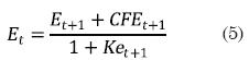
where E is the market value of equity, Ke is the levered cost of equity, and CFE, the cash flow to equity. CFE is defined as Div – ΔCS where Div is dividends paid and ΔCS is the change in capital stock.⁵ Dividends paid are what actually the equity holder receives from the firm and can put in the own pocket; ΔCS is the increase (new equity investment) or decrease (repurchase of equity) in CS, Capital Stock.

Model (5) is a standard in valuation of cash flow (see, for example, Miller and Modigliani, 1961, eq. (2)). However, we would like to explain in detail the reason for Et+1 in the model. What the market does to value a stock is to discount the full stream of dividends from t+1 to ∞. As we cannot model that fact, we can assume that for year t+1 the market did exactly the same but from t+2 to ∞. This is captured in the value of the stock (or market capitalization) for year t+1. Hence, when we include the dividends for year t+1 plus the market value at t+1, it is equivalent to having the full infinite stream of dividends from t+1 to ∞. That is what supposedly the market does. This is an incontrovertible formulation of the basic concept of time value of money and it is common knowledge.

From the previous model we have designed an econometric model to test our hypothesis. The correct model is:

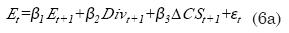
What we are doing when using this model is to see the value of the firm from the point of view of the share holders. We have a model that values the equity, and hence the terms in the right hand side (RHS) of (6a), including the cash flow to equity, CFE and the value of equity in t+1. What eq. (6a) indicates is exactly the same as eq. (5) does. The difference is that instead of having a common discount rate, Ke, we consider that each element of the CFE might have a different discount rate. The common term (1/(+ke)) a discount factor) is broken down into three discount factors represented by the β’s.

The definition of CFE in this model is clear and concise, and also supported by others authors. As Penman (2007) underlines,

Owner’s equity increases from value added in business activities (income) and decreases if there is a net payout to owners. Net payout is amounts paid to shareholders less amount received from share issues. As cash can be paid out in dividends or share repurchases, net payout is stock repurchases plus dividends minus proceeds from share issue [italics in original]. (p.39)

He also writes that “it is noncontroversial that the price of a security is expressed as the ‘present value’ of the expected future payoffs to holding the security” (Penman, 1992, p. 466), where “payoffs” unambiguously refers to “the payoffs for equity securities” (p. 466). His notions of “net cash flow to shareholders” (p. 239) or “net dividend” (p. 241) are consistent with our notion of cash flow to equity:

Net dividend= Cash dividend +Share repurchases–Share Issues

In order to test the hypothesis that ΔLA, the change in liquid assets, is irrelevant or destroys value, we falsify the correct model introducing the change in liquid assets, ΔLA, as follows:

In the two previous equations ΔCS corresponds to change in Capital Stock (in the data we have changed the sign to the change in CS: an increase in CS means extra investment from the equity holders and it is an outflow; a decrease in CS means a buyback of stocks and it is an inflow to the share holders), Div is dividends paid, ΔLA is undistributed potential dividends and equal to the change in liquid assets as shown above in equations (1) to (4). E means equity market value, and LA is liquid assets. In this model a proprietary approach is followed, where E_t is measured as the declared market capitalization.

This model is consistent with the standard finance theory, but we do not intend to claim that it is fully explanatory, nor we try to make use of it for forecasting purposes. The models are meant to provide information on the relevance of the independent variables, in particular, the relevance/irrelevance of ΔLA_t+1 to value creation. To this end, the various betas are to be interpreted as the discount factors for the independent variables. In particular, β4 is the discount factor for change in liquid assets, i.e. it represents the value at time t of one dollar of ΔLA_t+1 available at time t+1.

Coefficients for the variables are interpreted as follows: an increase of $1 in any variable will be equivalent to an increase of $β in value in t. If Β>0 (let us say, 0,80) then we say that one increase of $1 in a given variable (in t+1 ) it is equivalent to an increase of 0,80 of the value in t. The coefficient is a discount factor that brings back to t (present value) that $1 in t+1. This is exactly what we teach about the time value of money in our courses. On the contrary, if β<0 (in particular β₄, the coefficient for ΔLA in the falsified model) it means that it destroys value. Hence, if ΔLA decreases (negative) and its coefficient is negative, at the end it would mean that it creates value instead of destroying value. The logic of this lies in the fact that if we invest the funds in cash in hand or in a very low return investment, shareholders will push the management to distribute that money instead of leaving it, say, in the bank. They consider that they can invest it at a higher rate.

What do we expect from coefficients β? We expect β₁ and β₂ to be positive and less than 1. We expect β₄ to be zero or negative. We expect β₃ to be negative or positive. This last comment deserves an explanation: as CS is depicted as a cash flow, when it has a negative value it means that the shareholders have increased their investment in the firm. When it is positive it means that the firm has bought some equity back and it is an inflow for the equity holders. If β₃ is negative, it indicates that the market is recognizing a value driver in the extra equity investment: this means that -$1 of equity investment in t+1 is equivalent to-β₃ today, and this is a positive value (–β₃ × -$1). At the same time it would imply that the market sees the repurchase of equity as a negative value driver, even if it represents an inflow to the equity holder. On the contrary, if β₃ is positive, it would mean that the market values equity repurchases as a value driver, and is not aware that a new equity investment might be a value driver.

In order to normalize the data and avoid problems of size, currency, time, etc., we will divide each variable by the book value of total equity (BVE) in t. We also deflate items in year t+1 with the corresponding inflation rate. As all variables will be divided by book value of total assets, the ratio E/BVE will represent Tobin’s Q. These independent variables are the normalized proxies for components of equation (5).

Equations (6a) and (6b), the correct model, will be affected by BVE and deflated by (1+π_t+1) where p is inflation rate as follows:

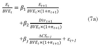
The falsified correct model is modified as follows:

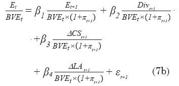
where all variables are now meant to be divided by book value of equity, the independent variables are also deflated. The deflation is made with Π_t+1, the inflation rate for year t+1. With this model, the value of the firm depends on the cash flows the owners of equity expect to receive in the future, and on potential dividends as well.

The components of model (7a) and (7b) depict the shareholders’ prospect of future value and cash flows to equity. The dependent variable is Tobin’s Q, w hereas the independent variables will be a percent of the book value of equity in t. With this model we try to measure how much value is created for a given value of the independent variables in the following period.

It should be here noticed that the models do not include an intercept. The reason is that we start from a correct financial and theoretical model. When we use an intercept it is because we fish out variables until we have come to a proper model. In this case, we repeat, we do not fish out variables. The variables are those stipulated by the correct model. In the falsified model we introduce a new (“strange” to the model) variable as they do in practice and recommend according to the literature review. And our hypothesis is that this new variable should be non-statistically significant.

2.2. The hypotheses

Our hypothesis may be phrased in a strong or in a soft version (similar to Vélez-Pareja and Magni, 2009):

“Strong version: we expect β₆ [or β₄ in this article] to be statistically zero (or close to zero). This means that investors will try to set down the value of Div_pot(t+1)[or ΔLA_t+1 in this article] by discounting it with an infinite, or at least at a very high discount rate, because they do not consider (undistributed) potential dividends relevant for valuation. Another condition might be that β₆ [or β₄ in this article] be negative and this would mean that potential dividends destroy value.

Soft version: we expect Div_pot(t+1)[or LAt+1 in this article] to be evaluated much less than the actual dividends. In econometric terms, we expect β₆ [or β₄ in this article] to be much smaller than β₅ [or β₃ in this article]” (pp. 145-146). A negative β₄ is included in the soft version of our hypotheses and this would mean that potential dividends destroy value. In terms of NPV, it means that investment in liquid assets does not have a zero NPV.

3. DESCRIPTION OF DATA

The source of data was primarily Economatica, and in case of abnormal behavior of the data we double checked with other sources. Secondary sources for checking purposes and completion of missing data were:

1. Google Finance: http://finance.google.com/finance
2. Argentina: Comisión Nacional de Valores, CNV (National Exchange Commision): http://www.cnv.gov.ar/
3. Brasil: BOVESPA (São Paulo Stock Exchange): http://www.bmfbovespa.com.br/home.aspx?idioma=pt-br
4. México: Bolsa Mexicana de Valores (Mexican Stock Exchange): http://www.bmv.com.mx/
5. Chile: Bolsa de Comercio de Santiago de Chile (Chilean Stock Exchange): http://www.bolsadesantiago.com/
6. Peru: Bolsa de Valores de Lima (Peruvian Stock Exchange): http://www.bvl.com.pe/

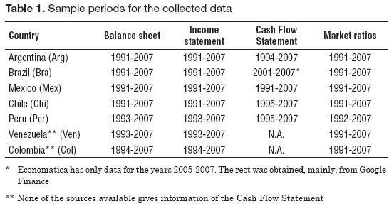
Initially we intended to collect data from seven countries, but the information for Colombia and Venezuela lacked of a very relevant variable: the actual dividends paid per year listed in the cash flow statement. In the case of Brazil we found in Economatica the dividends paid data for only three years. We completed for three more years using data from Reuters, Bloomberg and Google Finance.

Hence, we collected the data for five Latin American countries from 1991 to 2007. The countries with consistent and reliable data were: Argentina, Brazil, Chile, Mexico, and Peru. In particular we required that the data were directly available. The status of the information by country is like in Table 1.

For the implementation of the test, we collected information which is usually publicly available:

1. Market capitalization as declared by the firm with no adjustment for splits
2. CS = (Cumulated) capital stock contributed by shareholders
3. Div = Dividends paid in cash
4. C = Cash
5. STI = Short-term investments (marketable securities)
6. BVE = Book value of equity

With these data we calculated ΔCS, the change in capital stock and ΔLA the change in liquid assets (C+STI).

We had to fix some criteria to define how we would extract the data from the database, as follows:

1. Closing date: we found diverse dates for the fiscal year of the financial statements. However, all data were collected on December 31st. We have assumed that at this date there would be no signaling effect from dividends announcements.
2. The use of consolidated or not consolidated financial statements: we decided to use consolidated financial statements.
3. Currency and inflation adjustments: we extracted the financial statements in the local currency and without adjustments for inflation. The model provided “normalization” of the data dividing by BVE and deflating future values (in t+1) to the present period, t.
4. Dividends paid in cash: we decided to include in the sample only those firms (and countries) that reported the dividends effectively paid in cash in the cash flow statement. This was the reason why Colombia and Venezuela were excluded from the sample.

In our analysis we only included non financial firms and stocks with a high market liquidity index. The financial industry (banks, insurance firms, and pension funds) was excluded because we do not have dividends paid from the cash flow statement. Additionally, there is not a clear cut distinction between cash in hand and cash as an inventory to operate. The concept of liquid assets in the financial firms is somewhat different from the non financial firms. In the financial firms cash plays a different role as in non financial firms. We could even say (although it is not part of the study) that, by definition, financial firms do not hold liquid assets (CDs, pension funds investments, etc.). Cash in the financial firms plays the role of inventory.

We cleaned up the data and eliminated all those cases that did not have information for some of the variables. We distinguish between no data and zero as value of the variable. The result of this cleaning up was that the final sample was seriously unbalanced. See Appendix A for a complete description of the data collected.

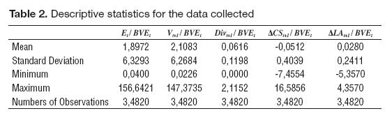
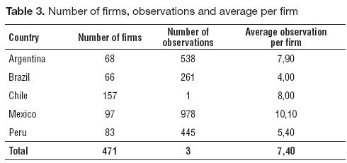
A statistical description of the collected variables follows including the deflation of terms in t+1 for the total sample is in Table 2. Composition of the data by country, number of firms and observations is displayed in Table 3.

4. RESULTS

In this section we show the different regression analyses performed with the data collected.

We have run several tests to measure the consistency and robustness of the data:

1. Homoscedasticity: we applied a test for robustness and it eliminated some variables from the model
2. Autocorrelation (passed)
3. Data panel that eliminated the same variables as in 1

The sequence of tests applied to the data is shown in Appendix B. The results for the models after the test for robustness follow. Table 4 shows the statistics for the falsified model. Notice we are including the potential dividends, as Damodaran calls them. As can be seen in Appendix B, first we tested a model including the constant or intercept. It also can be noticed here, that the constant is not significant. The final results after applying the robustness test are in Table 4.

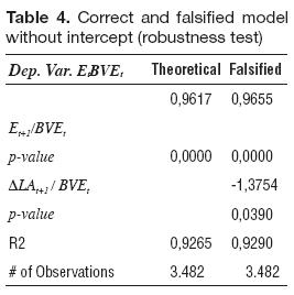
As we can see, β₄, the coefficient for ΔLA_t+1/BVE_t, is significant and has negative sign. This behavior of ΔLA_t+1/BVE_t, is identical in all regressions (with robust adjustment) excluding (one by one) the extreme values for E_t/BVE_t, that are greater than its mean plus three standard deviations. This is what was expected to happen and we can see the trend in Exhibit A4, in Appendix A.

We ran data panel tests for the correct and falsified models with and without intercept. The test for the two models with random effects, maximum likelihood effects (MLE) and without intercept, is displayed in the Table 5.

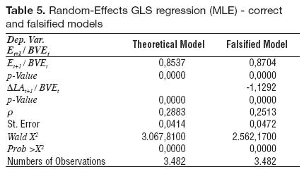
We can observe once again that E_t+1/BVE and ΔLA_t+1/BVE_t are significant at 5%.

In summary, we show the results with OLS with the robustness test and Data Panel with MLE in Table 6.

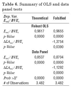
We can observe that ΔLA is statistically significant and its coefficient is negative. We must say that we have tested the model with the data that included the highest fifteen values (one by one) above the mean of the dependent variable plus 3-sigma and in all the tests ΔLA is consistently statistically significant and negative. Our sample included all the valid values; we did not delete any outlier. Our conclusion is that funds kept in cash and/or in short term investments destroy value as expected. This compares with some current literature mentioned in section one that assigns a positive value today or even greater than 1 to one dollar of liquid assets in next year. As it can be noticed we can say that the market is averse to the ΔLA as a value driver because β₄ is negative. The behavior of the coefficient for ΔLA deserves more explanation. In the strong version of our hypothesis we consider that ΔLA should not make any difference in value because ΔLA IS NOT a cash flow. Not being a cash flow should not appear in the model, hence its coefficient should be zero. When we falsify the model and insert that variable in it, we are testing the consequences of having some extra cash (or quasi cash) tied in the bank account or in short term investments. The data show that precisely the amount of funds tied to those items in the balance sheet are correlated to a lower (or loss of) value. This is what a negative coefficient for ΔLA means.

In tests using OLS and robust estimates with data within ±14 standard deviations dividends are statistically significant but the value of the coefficient is greater than 1, which is contrary to the financial theory of time value of money, although this result is consistent with the reported findings mentioned in the literature review.

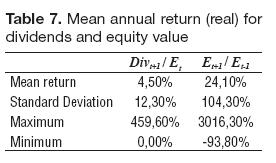
Moreover, we see that ΔLA destroys value, since each dollar in ΔLA in t+1 destroys -$1,13 of value today. The rejection of Div and ΔCS might be interpreted as if the market did not value dividends and that the market did not fully measure the impact of that extra investment in the value of the stock. What market values most is the expected value of E. One possible explanation is shown in Table 2 where, on average for the dividends (0,06 on the average) and ΔCS (-0,05 on the average) are so low compared with equity (1,90 on the average) that seems that the market does not value dividends as value drivers. In Table 7 we can observe the return on equity market value. In other words, our strong version hypothesis is rejected and this means that the Net Present Value of the investment in liquid assets is not zero, contrary to what generalized knowledge says.

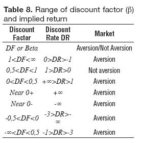
Now we analyze selected ranges for the discount factor, DF, and out of this point we can infer selected ranges for the implicit discount rate, DR. We constructed the Table 8 of Aversion / Not aversion by the market and values of the discount rate and factor.

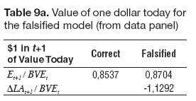
The meaning of the coefficients, as we have said before, is a discount factor that implies a discount rate. In Table 9a we show the discount factor for the correct model for the independent variables and for ΔLA from the falsified model.

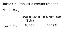
In terms of discount rates for each of the components of the CFE we can say that the implicit cost of equity for each component is:

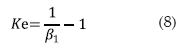
Implicit discount rates are shown in Table 9b.

In the same fashion, β₄, the coefficient of ΔLA_t+1/BVE_t implies a discount rate of -188,55%. This is an expected result and it might be interpreted as an aversion from the market to the potential dividends.

We examined the consistency of the coefficients and observed values for the theoretically correct model. We assume that the equity value can be calculated either considering each element of equation (1) has a discount rate, or that the sum of them (E_t+1 + CFE_t+1) has a single discount rate (Ke). The weighted average of betas (discount factor) is A, as follows:

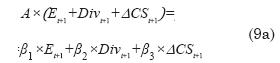
Equation (9a) means that in the model we assign a beta (a discount factor) to each component of equation (6a) in the RHS. In the left hand side (LHS), we consider the three elements of equation (6a) as a whole and discount it with an average discount factor, A.

The weighted average of betas should be the average discount factor for Ke. In this case we accept it is a proper discount factor if:

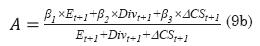
And restricted to 0<A<1, where A is the average discount factor for the correct model. An analysis of the values for A gives the following results (Table 10).

This mean implicit Ke compares with the implicit Ke in the coefficient of 17% and with the mean return of 24%.

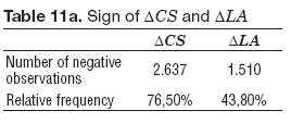
What is the behavior of the change in Capital Stock and Liquid Assets? This is relevant because it gives us an idea of the sign of the cash flow. A negative sign in ΔCS means that shareholders increased their invested capital. A negative sign in ΔLA means that the firm recovered investment in market securities and cash to use it in alternative investments or distributed it to the claim holders. In Table 11a we show the number of cases in the sample that have negative observations.

The sum of the ΔCS and ΔLA gives an idea of the relevance of the data (negative or positive) in the results. This is shown in Table 11b.

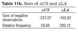
When we observe the results in the previous tables we conclude that almost 77% of the observations show an increase in capital stock. And not only this, the absolute amount is much larger that the buybacks (237,07 vs. 58,66). The fact that the change in capital stock has been rejected from the model could be interpreted as if the market does not recognize that the increase in capital stock represents an opportunity to increase the value of the firm.

On the other hand, we can see that the decrease in liquid assets is much lower, almost 44%. In this case, the absolute value of decreases compared with the increased is much lower: (102,62 vs. 200,12). The fact that change in liquid assets is rejected from the model might be interpreted as if the market perceives an increase of liquid assets as a value destroyer.

As a summary:

1. We have chosen a model that is robust and that has been long time ago supported by current literature and practice. It is based on the findings of Modigliani and Miller (1958, 1963). The model is common to all present value analysis. We have tested a well proven and utilized model in the current financial valuation practice.
2. The model is statistically significant and has an R² of at least 0,92.
3. We have analyzed a database that is significant: 3.482 observations.
4. Given the linear structure of the model, we consider that OLS is an appropriate estimation tool for the model. We tested the regression results with additional tests such as autocorrelation⁶ and homoscedasticity. As a final test we applied data panel to test the data.
5. Given that the model is theoretically correct, we have not added any additional independent variable. The model has only the variables included in the correct version. We have falsified the correct model with an independent variable that is used precisely for testing its relevance. We tested the intercept and it proved to be non significant.
6. Our prior expectation before gathering and analyzing the available data is partially confirmed with the analysis. The model was proposed in Vélez-Pareja and Magni (2009).

5. CONCLUDING REMARKS

We have found the empirical evidence that liquid assets destroy value. This confirms Jensen’s (1986) free cash flow agency problem. We also found that the investment in liquid assets is not perceived by the market as a zero NPV investment.

On the other hand, we found that the market discounts the CFE with discount rates below 100%. Contrary to what is found in some literature, one dollar in the future is worth less than one dollar today as expected according to the time value of money concept.

In summary, we can draw several conclusions:

1. This exploration is a confirmation of the Jensen’s (1986) free cash flow agency costs problem. Excess cash should be distributed because its retention destroys value.
2. Investment in liquid assets does not have a zero NPV. It has a negative NPV.
3. Market values more the expected price of the share than dividends. In fact, the independent variable Dividends (Div) is rejected from the regression.
4. Analysts should not include change in Liquid Assets (LA) as cash flow, because it is a fiction that contradicts the empirical evidence of reality.
5. There is an overvaluation of cash flows when the analysts include in the value the actual book value of liquid assets when it is assumed that liquid assets are zero NPV investments. While the change in liquid assets is discounted at the cost of capital when included in the FCF, that change, with contrary sign is discounted at usually a lower rate when considered as part of the cash flow of the liquid assets investment.
6. If analysts include ΔLA in the cash flow, this is to say that ΔLA is fully distributed, it should be consistency between the financial statements and the cash flows. In other words, the equity book value should show the fact that there is either a new equity investment, or a repurchase of equity.

The fact that idle cash or cash invested in low return investments destroys value is not solved by including those amounts that are listed in the balance sheet in the cash flows as if they were distributed to shareholders. The solution is to effectively distribute the funds to them.

As a practical and general conclusion, the empirical evidence suggests that we should include in the working capital the liquid assets, as well as eliminate the practice of adding the book value of liquid assets under the assumption that they are zero NPV investments. The only relevant cash flow is what effectively an investor receives from the equity investment: dividends and stock repurchases.

Our conclusions are in line with the thinking of DeAngelo and DeAngelo (2006, 2007), who have devoted much of their researches mainly explaining that only distributed cash flows produce value.

FOOTNOTES

1. Este documento fue seleccionado en la convocatoria para enviar artículos, Call for Papers, realizada en el marco del Simposio “Análisis y propuestas creativas ante los retos del nuevo entorno empresarial”, organizado en celebración a los 30 años de la Facultad de Ciencias Administrativas y Económicas de la Universidad Icesi y de los 25 años de su revista académica, Estudios Gerenciales; el 15 y 16 de octubre de 2009, en la ciudad de Cali (Colombia). El documento fue presentado en las sesiones simultáneas del área de “Finanzas”.

2. Eqs. (1) and (3) may obviously be written as:

3. From equation (1) to this point it has been taken and adapted from Vélez-Pareja and Magni (2009).

4. Professor Tom Copeland in a private correspondence says (August 6th, 2004): “If funds are kept within the firm you still own them -hence ‘potential dividends’ are cash flow available to shareholders, whether or not they are paid out now or in the future.”

5. ΔCS from the point of view of the equity holder, is positive when the firm buybacks equity and negative when the equity holder invests additional funds in the firm.

6. Some tests cannot be applied, such as the Granger Test because we need a time series and our data have under the best of circumstances a sequence of 11 observations and it can be applied only to pairs of variables. See Appendix A, "Table A4.

BIBLIOGRAPHIC REFERENCES

1. Benninga, S. (2006). Principles of Finance with Excel. London: Oxford.        [ Links ]

2. Benninga, S.Z. and Sarig, O.H. (1997). Corporate Finance. A Valuation Approach. New York, NY: McGraw-Hill.        [ Links ]

3. Brealey, R. and Myers, S.C. (2003). Principles of Corporate Finance (7th ed.). New York, NY: McGraw- Hill-Irwin.        [ Links ]

4. Chu, H. and Partington, G. (2008). The Market Valuation of Cash Dividends: The Case of the CRA Bonus Issue. International Review of Finance, 8(1-2), 1-20. Available at SSRN: http://ssrn.com/abstract=1138832 or DOI: 10.1111/j.1468-2443.2008.00072.x        [ Links ]

5. Copeland, T.E., Koller, T. and Murrin, J. (1990). Valuation: Measuring and Managing the Value of Companies. New York, NY: John Wiley & Sons.        [ Links ]

6. Copeland, T.E., Koller, T. and Murrin, J. (1994). Valuation: Measuring and Managing the Value of Companies (2nd ed.). New York, NY: John Wiley & Sons.        [ Links ]

7. Copeland, T.E., Koller, T. and Murrin, J. (2000). Valuation: Measuring and Managing the Value of Companies (3rd ed.). New York, NY: John Wiley & Sons.        [ Links ]

8. Damodaran, A. (1999). Applied Corporate Finance. A User’s Manual. New York, NY: John Wiley & Sons.        [ Links ]

9. Damodaran, A. (2005). Dealing with Cash, Cross Holdings and Other Non-Operating Assets: Approaches and Implications. Available at SSRN: http://ssrn.com/abstract=841485        [ Links ]

10. Damodaran, A. (2006a). Damodaran on Valuation (2nd ed.). Hoboken, NJ: John Wiley & Sons.        [ Links ]

11. Damodaran, A. (2006b). Valuation approaches and metrics: a survey of the theory and evidence. Available at SSRN: <http://www.stern.nyu.edu/~adamodar/pdfiles/papers/valuesurvey.pdf> Originally published in Foundations and Trends® in Finance, 1(8), 693-784, 2005.        [ Links ]

12. Damodaran, A. (2008). Equity instruments: Part I. Discounted cash flow valuation. Recovered on January 3, 2009, from: www.stern.nyu.edu/~adamodar/pdfiles/eqnotes/packet1.pdf (updated January 14, 2008).        [ Links ]

13. DeAngelo, H. and DeAngelo, L. (2006). The Irrelevance of the MM Dividend Irrelevance Theorem. Journal of Financial Economics, 79, 293–315. Available at SSRN: http://ssrn.com/abstract=680855 or DOI: 10.2139/ssrn.680855        [ Links ]

14. DeAngelo, H. and DeAngelo, L. (2007). Payout policy pedagogy: what matters and why. European Financial Management, 13(1), 11-27.        [ Links ]

15. Dechow, P.M., Richardson, S.A. and Sloan, R.G. (2006). The Persistence and Pricing of the Cash Component of Earnings. 20th Australasian Finance and Banking Conference 2007 Paper. Available at SSRN: http://ssrn.com/abstract=638622        [ Links ]

16. Faulkender, M.W. and Wang, R. (2004). Corporate financial policy and the value of cash (working paper). Available at SSRN: http://ssrn.com/abstract=563595        [ Links ]

17. Fernández, P. (2002). Valuation Methods and Shareholder Value Creation. San Diego, CA: Academic Press.        [ Links ]

18. Fernández, P. (2007). Company valuation methods. The most common errors in valuation (working paper). Available at SSRN: <http://ssrn.com/abstract=274973>.        [ Links ]

19. Harford, J. (1999). Corporate cash reserves and acquisitions. Journal of Finance, 54(6), 1969-1997. Recovered in January 30, 1997, from: http://ssrn.com/abstract=2109        [ Links ]

20. Jensen, M.C. (1986). Agency cost of free cash flow, corporate finance, and takeovers. American Economic Review, 76(2), 323-329. Available at SSRN: http://ssrn.com/abstract=99580 or DOI: 10.2139/ssrn.99580.        [ Links ]

21. Mikkelson, W.H. and Partch, M. (2003). Do persistent large cash reserves lead to poor performance? Journal of Financial and Quantitative Analysis, 38(2), 275- 294. Available at SSRN: <http://ssrn.com/abstract=186950> or DOI: 10.2139/ssrn.186950.        [ Links ]

22. Miller, M.H. and Modigliani, F. (1961). Dividend policy, growth and the valuation of shares. The Journal of Business, 34(4), 411- 433.        [ Links ]

23. Modigliani, F. and Miller, M.H. (1958). The cost of capital, corporation taxes and the theory of investment. American Economic Review, 47, 261-297.        [ Links ]

24. Modigliani, F. and Miller, M.H. (1963). Corporate income taxes and the cost of capital: a correction. American Economic Review, 53, 433-443.        [ Links ]

25. Opler, T.C., Pinkowitz, L., Stulz, R.M. and Williamson, R. (1999). The determinants and implications of corporate cash holdings. Journal of Financial Economics, 52(1), 3-46. Available at SSRN: http://ssrn.com/abstract=225992        [ Links ]

26. Penman, S. (1992). Return to fundamentals. Journal of Accounting, Auditing and Finance, 7, 465-483. Reprinted in R. Brief and K.V. Peasnell (Eds.), Clean Surplus: A Link Between Accounting and Finance. New York and London: Garland Publishing.        [ Links ]

27. Penman, S. (2007). Financial Statement Analysis and Security Valuation (3rd ed.) New York, NY: McGraw-Hill.        [ Links ]

28. Penman, S. and Sougiannis, T. (1998). A comparison of dividends, cash flow, and earnings approaches to equity valuation. Contemporary Accounting Research, 15(3), 343- 383.        [ Links ]

29. Pinkowitz, L., Stulz, R.M. and Williamson, R. (2003). Do firms in countries with poor protection of investor rights hold more cash? (Dice Center working paper No. 2003-29). Available at SSRN: http://ssrn.com/abstract=476442 or DOI: 10.2139/ssrn.476442.        [ Links ]

30. Pinkowitz, L. and Williamson, R.G. (2002). What is a dollar worth? The market value of cash holdings (working paper). Available at SSRN: http://ssrn.com/abstract=355840 or DOI: 10.2139/ ssrn.355840.        [ Links ]

31. Pinkowitz, L., Williamson, R. and Stulz, R.M. (2007). Cash holdings, dividend policy, and corporate governance: a cross-country analysis. Journal of Applied Corporate Finance, 19(1), 81-87.        [ Links ]

32. Schwetzler, B. and Carsten, R. (2003). Valuation effects of corporate cash holdings: Evidence from Germany. HHL (working paper). Available at SSRN: http://ssrn.com/abstract=490262        [ Links ]

33. Shrieves, R.E. and Wachowicz, J.M. (2001). Free Cash Flow (FCF), Economic Value Added (EVA), and Net Present Value (NPV): A Reconciliation of Variations of Discounted- Cash-Flow (DCF) Valuation. The Engineering Economist, 46(1), 33-52.        [ Links ]

34. Tham, J. and Vélez-Pareja, I. (2004). Principles of Cash Flow Valuation. Boston, MA: Academic Press.        [ Links ]

35. Vélez-Pareja, I. (1999a). Construction of free cash flows: a pedagogical note. Part I (December) (working paper). Available at SSRN: http://ssrn.com/abstract=196588        [ Links ]

36. Vélez-Pareja, I. (1999b). Construction of free cash flows: a pedagogical note. Part II (December) (working paper). Available at SSRN: http://papers.ssrn.com/sol3/papers.cfm?abstract_id=199752        [ Links ]

37. Vélez-Pareja, I. (2004). The correct definition for the cash flows to value a firm (free cash flow and cash flow to equity) (working paper). Available at SSRN: http://ssrn.com/abstract=597681        [ Links ]

38. Vélez-Pareja, I. (2005a). Once more, the correct definition for the cash flows to value a firm (free cash flow and cash flow to equity) (Working Paper). Available at SSRN: <http://ssrn.com/abstract=642763>.        [ Links ]

39. Vélez-Pareja, I. (2005b). Construction of cash flows revisited (working paper). Available at SSRN: <http://papers.ssrn.com/sol3/papers.cfm?abstract_id=784486>.        [ Links ]

40. Velez-Pareja, I. and Magni, C.A. (2009). Potential dividends and actual cash flows in equity evaluation. A critical analysis. Estudios Gerenciales, 25(113), 123-150.        [ Links ]

ONLINE REFERENCES

41. Bolsa de Comercio de Santiago de Chile (Chilean Stock Exchange): http://www.bolsadesantiago.com/. Visited on May 23, 2008.        [ Links ]

42. Bolsa de Valores de Lima (Peruvian Stock Exchange): http://www.bvl.com.pe/ . Visited on May 23, 2008.        [ Links ]

43. Bolsa Mexicana de Valores (Mexican Stock Exchange): http://www.bmv.com.mx/. Visited on May 23, 2008.        [ Links ]

44. BOVESPA (São Paulo Stock Exchange): http://www.bmfbovespa.com.br/home.aspx?idioma=pt-br        [ Links ]

45. Comisión Nacional de Valores, CNV (National Exchange Commision): http://www.cnv.gov.ar/. Visited on May 23, 2008.        [ Links ]

46. Google Finance: http://finance.google.com/finance. Visited on May 23, 2008.        [ Links ]