


Services on Demand
Journal
Article
 English (pdf)
 Article in xml format
 Article references
 Send this article by e-mail
Indicators
-
 Cited by SciELO
 -
 Access statistics
Related links
-
 Cited by Google
 -
 Similars in
SciELO
Similars in
SciELO -
 Similars in Google
Share

 Permalink
Estudios Gerenciales
Print version ISSN 0123-5923
estud.gerenc. vol.26 no.114 Cali Jan./Mar. 2010
DIFFERENT IMPACT CHANNELS OF EDUCATION ON POVERTY1
BLANCA ZULUAGA DÍAZ
PhD in Economics (candidate), Universidad Católica de Lovaina, Bélgica. Profesora tiempo completo, Departamento de Economía, Universidad Icesi, Colombia. Grupo de investigación "Economía, políticas públicas y métodos cuantitativos", Universidad Icesi, Colombia. Grupo de Economía Pública – CES, Universidad Católica de Lovaina, Bélgica. Dirigir correspondencia a: Universidad Icesi, Calle 18 No. 122-135, Cali, Colombia. bzuluaga@icesi.edu.co
Fecha de recepción: 20-11-2008 Fecha de corrección: 23-07-2009 Fecha de aceptación: 18-01-2010
ABSTRACT
This article analyzes both the monetary and non-monetary effects of the education level of the head of the household on poverty. We propose that schooling returns should not be thought as a single number - usually the schooling coefficient in an income equation - but as a set of elements whose length depends on the number of identified poverty dimensions. The monetary analysis employs the Quantile Regression technique, very helpful especially when one is interested in extremes of the income distribution function. Our results show differences across quantiles of the returns. We also found interesting dissimilarities by gender and urban-rural location. Exploring the non-pecuniary returns, we found that the education of the head positively influences family health and housing conditions.
KEYWORDS
Returns to education, poverty, quantile regression.
Clasificación JEL: I20, I30
RESUMEN
Canales de impacto de la educación en la pobreza
En este artículo se analizan los efectos monetarios y no monetarios que tiene en la pobreza el nivel de educación del jefe de familia. Se plantea que los retornos a la educación no deben ser vistos como una cifra–generalmente un coeficiente de educación en una ecuación para el cálculo de los ingresos– sino como una serie de elementos cuya duración depende del número de aspectos identificados de la pobreza. Se utilizó la técnica de regresión por cuantiles, la cual es útil cuando se está interesado en los extremos de la función de distribución de ingresos. Los resultados demuestran diferencias entre los cuantiles de los retornos. Se encontraron diferencias interesantes por género y ubicación rural/urbana. Una exploración de los retornos no pecuniarios reveló que la educación del jefe de familia influye positivamente en las condiciones de salud y vivienda de la familia.
PALABRAS CLAVE
Retornos a la educación, pobreza, regresión por cuantiles.
RESUMO
Differentes canais de impacto da educação na pobreza
O artigo analisa os efeitos monetários e os não-monetários do nível de escolaridade do chefe de família na situação de pobreza. Propomos que o rendimento da escolaridade não seja pensado como um simples número– usualmente o coeficiente de escolaridade em uma equação da renda–mas como um conjunto de elementos cuja extensão depende da quantidade de dimensões de pobreza identificadas. A análise monetária usa a técnica de Regressão Quantil, muito útil especialmente quando estamos interessados nos extremos da função de distribuição das rendas. Nossos resultados mostram diferenças entre os quantis dos retornos. Também encontrámos interessantes desigualdades conforme o sexo e a localização urbana-rural. Explorando os retornos não pecuniários, descobrimos que a educação do chefe de família influencia positivamente a saúde familiar e as condições de habitação.
PALAVRAS CHAVE
Retornos da educação, pobreza, regressão quantil.
INTRODUCTION
The academic discussion about the benefits of schooling in increasing the welfare of individuals is very extensive and methodologically diverse. Researchers have emphasized the importance of education to: i) increase the ability of individuals to acquire higher income, and ii) positively influence several social and economic outcomes that improve people’s wellbeing, this is, returns to education have multiple dimensions. For instance, Haveman and Wolfe (1984) present an enriched list containing different impact channels of schooling including private and public effects, marketed and non marketed returns such us intra-family productivity, child quality - level of education and cognitive development of children-, family health, fertility, crime reduction, social cohesion, savings, income distribution, among other 20 channels of impact.
The need to privilege a multidimensional approach when measuring returns to education is aligned with the tendency in the literature to measure poverty and inequality in a multidimensional framework. According to this approach, income is only one of the multiple dimensions where an individual or household may experience poverty conditions (Sen, 1985) and only one of the several attributes on which it is interesting to analyze inequality. Indeed, authors like Atkinson and Bourguignon (1982), Bourguignon and Chakravarty (2003), Tsui (1994, 2002), among others, have focused their contributions in providing an appropriate methodology for the estimation of aggregate multidimensional poverty indices. Bourguignon and Chakravarty, for instance, suggest to specify a poverty line for each dimension; someone would be considered as poor if he falls below at least one of the defined poverty lines (union approach). The authors combine the different poverty lines and the corresponding gaps - difference between the observed outcome and the specified poverty threshold -, the result is a multidimensional measure of poverty.
Apart from the multidimensional nature of the educational returns, another relevant aspect when analyzing the benefits of schooling is that those returns may differ according to the type of individuals that are improving their human capital. This is, monetary and non-monetary returns to education are heterogeneous among groups, and it is interesting to explore such differences in order to more efficiently design educational policies as antipoverty policies.
This empirical article aims at estimating, using Colombian data, the returns to education related to various poverty dimensions and corresponding to different groups of individuals, differentiated essentially by gender, income quintile, and rural-urban location. We propose that, when analyzing education as an antipoverty policy, schooling returns should not be thought as a single number (usually the coefficient of schooling in an income or earnings equation) but as a set of elements whose length depends on the number of identified poverty dimensions. This is,
Where αij corresponds to the return to education in terms of dimension j=1, 2 n for the group of individuals (e.g men, women, poorest quintile of income distribution, etc). This method of estimating returns is useful to compare the relative impact of education on different vulnerable groups, say, women, inhabitants of rural areas, people from poor neighborhoods, among others. It also allows us to detect possible obstacles for certain educated groups to realize the benefits of education; for instance, comparing returns of women and men, one might find signals of failures in the economic environment that hinder women to enjoy their improved schooling level. We will see that our results do not validate this potential failure. Another reason why this presentation of the returns is useful is that we may identify certain type of individuals that are a better target for educational policies, since they obtain higher returns related to a given poverty dimension (for instance, women head of households and family health).
Even if it may seem restrictive, for this research we have chosen to use the information corresponding to the heads of households, because education of the heads plays a decisive role in shaping the socioeconomic characteristics of the household as a whole, hence, its poverty conditions. However, this means that we should be careful with the interpretation of our results, for instance when analyzing educational returns for female heads, since women’s headship is not a random or exogenous characteristic.
We are interested in exploring the different channels through which the level of education of the ‘head’ impacts the poverty level of the household they lead. We identify both monetary and non-monetary returns to education, which corresponds, respectively, to the effect of schooling on the income poverty dimension and its effect on other poverty dimensions like health and housing. When estimating the non-pecuniary returns, one of our main interests is to distinguish the impact of education and that of income on the specific outcome.
The pecuniary analysis employs the quantile regression technique (Koenker, 2005; Koenker and Bassett, 1978; Koenker and Hallock, 2001). This methodology is very helpful especially when one is interested in the lowest or highest extremes of the distribution function of the dependent variable. In fact, there is no reason to believe that the estimates of the effects of education on the income of households or individuals do not vary between the lowest and the upper tail of the income distribution. By using the traditional Least Square estimation, we would obtain only the effect of education on the conditional mean of the response variable. In contrast, quantile regression offers coefficient estimations for any conditional quantile.
Besides, given that education is an endogenous variable in the equation explaining the income level of the household, we use an instrumental variable quantile regression technique recently popularized by Chernozhukov and Hansen (2001, 2004, 2005) among others. Interesting findings are obtained when making the analysis by gender and (urbanrural) sector.
This article is organized as follows. The second section presents a short review of some contributions to the theory on educational returns that were relevant for this document. Besides, the methodology used to estimate the model is explained.
In the third section, we explain the data and show some descriptive statistics of the variables. In the fourth and fi fth sections we present the estimations of both pecuniary and nonpecuniary educational returns using Colombian data. The results of the instrumental variable quantile regression confirm the heterogeneity of the effect of education across quantiles of the conditional household-income distribution, specifically comparing the extremes of the income distribution. Moreover, the estimates reflect the relevance of the non-pecuniary effects, and confirm that an analysis based only on monetary outcomes is incomplete. Finally we present the conclusions.
1. THEORETICAL PRELIMINARIES AND METHODOLOGY
Let us start with the monetary effect of education on poverty, i.e. the income return to education. In the human capital literature, whose pioneers are Schultz (1961) and Becker (1965), education is seen as an investment of present resources (time opportunity cost and direct costs) in order to obtain future returns. Schultz argued that knowledge and skills are a form of capital, which is a result of deliberate investment. Education, training, and health investment, increase opportunities and choices available to individuals, by affecting the ability to do productive work. Schultz attributes the difference in earnings between people to the differences in access to education and health.
As for Becker (1965), he assumes that individuals choose education to maximize the present value of expected future incomes before retirement, net of the costs of education. Investing in education entails explicit costs (i.e. fee, books, transport, etc.) and implicit costs, corresponding to the opportunity cost of spending money and time on education instead of working to increase current income and production. The return of the nth year of education can be seen as the difference between the wage obtained with n years of schooling and the wage obtained with n-1 years of schooling. Based on this assessment, several estimations of schooling returns for different countries have been carried out by analyzing the variation of wages with an additional year of schooling.
An important extension of the human capital theory is made by Mincer (1974), which has been the benchmark for a great number of empirical work on labor economics and economics of education. Based on empirical and theoretical arguments, the Mincer equation expresses earnings as a function of schooling and experience. The simplest version of the Mincerean wage equation was followed by a number of extensions, among others by Hungerford and Solon (1987), whose main contribution was to highlight the non-linearity of the relationship between years of schooling and income described in the Mincer equation. Indeed, there exist the so-called `sheepskin effects’, which refl ect higher increments in wage in those years of schooling that represent the culmination of an educational level (i.e. secondary or higher).
In this article, we want to explore the effect of schooling level of the head of the household Shh in total household income Yh. The problem of endogeneity of the schooling variable should be solved in order to obtain consistent estimators. We then estimate,
Where we expect  to be exogenous, Z is a vector of instrumental variables related to and unrelated to income, and Xhh is a vector including other variables affecting household income. The idea is to identify exogenous infl uences on schooling decisions. Harmon and Walker (1995) exploit the exogenous changes in the distribution of education of individuals due to the increase of the minimum school-leaving age. Angrist and Krueger (1991) employ the season of birth of individuals to provide instruments for schooling. They consider the fact that those students born at the beginning of the year start education at an older age than students born at the end of the year. Therefore, the first group reaches school-leaving age earlier and may drop out after completing less schooling than individuals from the second group. Another example is Card (1993), who employs data on proximity to schools considering that individuals living close to an educational institution are more likely to attend school than those living far away.
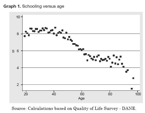
In line with Harmon and Walker (1995), we have explored exogenous variations on the schooling attendance of individuals in Colombia. Our instrument reflects the great educational expansion that Colombia experienced since the middle of the fifties. Due to the governmental purpose to universalize primary education, the years of schooling of that cohort of individuals and the next cohorts, increase significantly compared to earlier cohorts. This will be equivalent to considering a change in minimum school-leaving age to be equal to 12 years. Explicitly, the instrument is a dummy taking the value of 0 for people born before 1951 and equal to 1 for those born from that year on. Graph 1 shows the average schooling across cohorts, which is motivating the choice of the instrument.
The analysis of the impact of education on income offers more interesting insights if we can identify this influence on different quantiles of our response variable distribution - household income -. For such a purpose, a conventional Least Square regression is not helpful, since it only captures the relationship between covariates and the conditional mean of the dependent variable. In contrast, Quantile Regression, an alternative econometric method introduced by Koenker and Bassett (1978), captures the relationship between the covariates and any conditional quantile of the response variable. In our case, for instance, the method allows us to concentrate attention on the lowest income groups.
Following Koenker (2005), we have that, for a random variable Y with probability distribution function F(Y) = Pr (Y ≤ y) the  th thquantile of Y is,
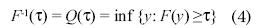
Thus, the median of a distribution corresponds to Q(0,5).
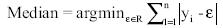
Recall that, for a random sample of Y , the sample median minimizes the sum of absolute deviations or residuals which means;
Similarly, the th sample quantile may be written as,
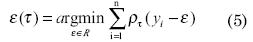
Where  I(.) is an indicator function equal to 1 if (yi–ε) < 0, equal to 0 otherwise. Now, the linear conditional quantile function,
Can be estimated as the solution of the th regression quantile β():
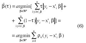
The traditional OLS method provides an estimate of β which expresses the relationship between X and the conditional mean of Y. In contrast, the use of quantile estimations allows us to obtain β() for any quantile  (0,1), this is, the relationship between X and any quantile of the distribution of Y.
Now, when we have to deal with an endogeneity problem, the right method to estimate the model is an Instrumental Variable Quantile Regression. Chernozhukov and Hansen (2001, 2004, 2005) deal with this issue. They worked out a model of quantile treatment effect - QTE - under endogeneity and obtain conditions for identification of the QTE without functional form assumptions. This technique is known as Instrumental Variable Model of Treatment Effect, which modifies the estimation procedure of the quantile regression by introducing instrumental variables that correct for the endogeneity problem and allow us to obtain consistent estimators.
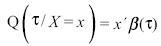
Based on Chernozhukov and Hansen’s methodology, in the next section we estimate the coefficients of the schooling variable by income quintile, which allows us to distinguish the effect of education among the poorest groups respect to the richest. The estimated conditional quantile models can be expressed as follows:
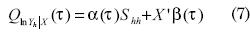
Where X is a vector of independent variables. As mentioned, an instrument for education reflecting a change in schooling leaving age is used.
Let us now focus on the non pecuniary effects of schooling. Certain decisions and the behavior of individuals might be favorably changed as education increases, allowing people to avoid or escape from poverty. Specifically, a higher capability to make more convenient - crucial - decisions increases the probability of success in reaching basic needs.
In the literature of the economics of education, there are important contributions on the non-market benefits of schooling such as Becker (1965), Michael (1972), Grossman (2005), and Haveman and Wolfe (1984), already mentioned in the introduction. The main idea of these contributions is that education positively influences the efficiency of non-market sector production processes (household production): consumers produce commodities using inputs and time, and education reduces the absolute and relative marginal costs of home produced commodities. It also influences certain decisions of individuals such as growth in consumption (savings) during the life cycle, quantity and quality of children, addiction to drugs, etc.
Grossman (2005) emphasizes the influence of education on the increase of both, production efficiency and allocative efficiency. To illustrate the first aspect, production efficiency, he uses the example of health, and concludes that an increase in schooling is predicted to increase the quantity of health demanded but to lower the quantity of medical care demanded. Intuitively, a combination of good habits and a greater valuation of health as one of the most important source of human capital, leads to this result. As for efficiency in allocation, more educated people are able to pick a better combination of inputs that gives them more quantity of output.
The focus in this article will be on the non- market benefits of education that are related to poverty, specifically, those educational impacts on basic needs. With this purpose, we will use reduced forms of a household production function of basic commodities that enter a utility function. Becker (1965) claimed that households, as utility maximizers, combine market goods (x) and time (T) to produce such commodities (j),
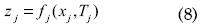
In our context, education is thought as an input entering the production functions of all the commodities that we are interested in analyzing. More specifically, z will represent health conditions, affiliation to the health system, and housing conditions.
There are several reasons to support reduced forms of (8) related to basic needs. Education enhances the ability to receive adequate nourishment: a well-educated person is more likely to select the right food needed to attain proper levels of nutrition, even with little money. Likewise, a person with higher education is better informed and therefore has the option to adopt good habits that allow him to have a healthier life. Knowledge of the human body, and its functioning, allows the person - if he wants - to take better care of it (Kenkel, 1991; Strauss, 1990).
A similar correlation with education applies to the capability to avoid premature mortality. In addition, the capability of family planning has an obvious link with education, as familiarity with the reproductive system and contraceptive methods may help people to prevent unexpected pregnancies (Michael and Willis, 1976). There is an impact on the desired number of children as well, for at least two reasons: higher opportunity cost of having children (forgone income for raising children is higher for an educated person) and preference for postponing the age to start breeding (while educational investment is taking place).
The results for the non-monetary effects of education that are shown in the next section come from an equation of the form:
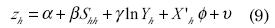
Where the response variable zh corresponds to health and housing outcomes. On the RHS we have schooling of the head (Shh), household income (lnYh), and other characteristics of the households and the head (vector X). We are interested in distinguishing the impact of education and that of income: differences in households’ outcomes are not exclusively explained by differences in income, but also by the schooling level of the head.
The Hausmann test revealed that both schooling and income are endogenous variables, hence, the error term is v = v + ε, i.e. the sum of an exogenous component and a component of unobserved factors related to the endogenous variables. Thus, we instrumented S by using, as before, a dummy reflecting changes in the school leaving age. In addition, we instrumented the variable income by using the regional unemployment rate, as suggested by Ettner (1996). Ettner claims that, in spite of the concern that the instrument may be correlated with health (high unemployment rates may be detrimental to mental health), the Wald tests do not provide consistent evidence to doubt the suitability of unemployment rate as an instrument - the variable satisfies the exclusion restriction-. Our own tests statistically justify the use of this variable as an instrument.
Before going to the results, it is worthy to notice that income gains of schooling are obtained only when agents have finished school and enter the labor market, while the nonmonetary gains might be perceived even before the schooling investment period has culminated.
2. DATA DESCRIPTION
We will employ micro-data from a Colombian database called "Quality of Life Survey". The sample design of the survey allows researchers to analyze the data at national level and by regions. The National Department of Statistics (DANE) carried out this survey in 1997 and 2003. The pooled cross section data contains information for 31.745 households. The survey inquires about housing conditions, access and quality of water, characteristics and composition of the household, health, characteristics of children less than five years old, education (to members five years old or more), employment, life conditions of the household, and household spending.
Table 1 summarizes the variables included in the estimated models. In the income equation, instead of the usual quadratic age variable, a quartic expression is considered. This is in line with the findings of Lemieux (2006), who argues that a quartic function better reflects the income - experience profile. In order to remove from the income returns any assortative mating effect of education, we control by including the schooling of the spouse in the income equation. Moreover, we also remove from the estimated returns the effect of education on family size, by including the variable dependency rate. Finally, as we are working with pooled cross section data, there is a dummy equal to zero if the information corresponds to 1997 and equal to 1 if it corresponds to 2003.
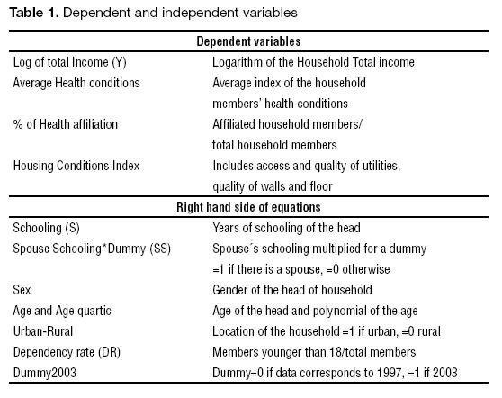
As for the non-pecuniary returns estimations, we use three dependent variables: percentage of affiliation to the health system, average health conditions of the household, and an index of housing conditions. The first health indicator corresponds to a simple rate between family members affiliated to the health system over the total family members. The second health indicator is obtained as follows: each member of the household has a given level of health conditions, labeled numerically from bad to excellent. The individual health conditions are averaged by household to obtain our dependent variable. These variables transformations are justified if we wanted to continue the analysis at the household level as in the previous section.
The housing conditions index is based on information about access and quality of utilities, material of walls and floor. For each variable involved we have three categories: bad/fair/good (never/sometimes/always in the case of access to utilities). We gave them numbers from 1 to 3, and add them up to obtain a single housing index. Thus, it is assumed that all the different attributes are equally important to define the index. As this method looks quite ad hoc, a principal component analysis (PCA) was used to check if results would differ.
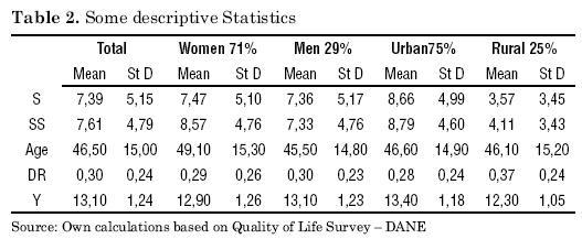
Table 2 shows some descriptive statistics of the data. The information shows a clear disadvantaged of the rural sector in all indicators: schooling of both heads of households and their spouses are lower than for any other group, as well as the average income, while the dependency rate is the highest. As for gender, income is slightly lower for women. There is no important difference in schooling years for male and female heads, but it is noticeable the difference in years of education among their wives and husbands.
3. MONETARY RETURNS TO EDUCATION
3.1. Results of the Instrumental Variable Quantile Regression
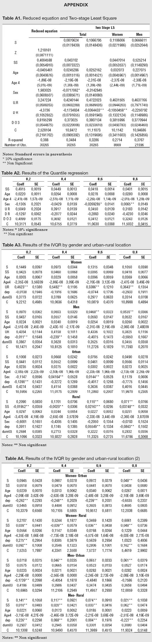
The income equation estimated here includes the following control variables: head schooling (instrumented), spouse schooling, age of the head, a polynomial of age, gender of the head, urban-rural location of the household, dependency rate, and a dummy indicating the year of the data. In the schooling equation or reduced equation, the instrument is significant and, as expected, has positive sign (see Table A1 in the appendix).
By using the Two- stage Least Square method we find that an additional year of schooling of the head of the household increases total income of the household by around 8,7% (see Table A1 in the appendix for the complete results).
There are interesting results when doing the regressions by quantiles:2 the schooling coefficient decreases as quantile increases. The educational return for the lowest quintile doubles the return corresponding to the highest quintile (see Graph 2).
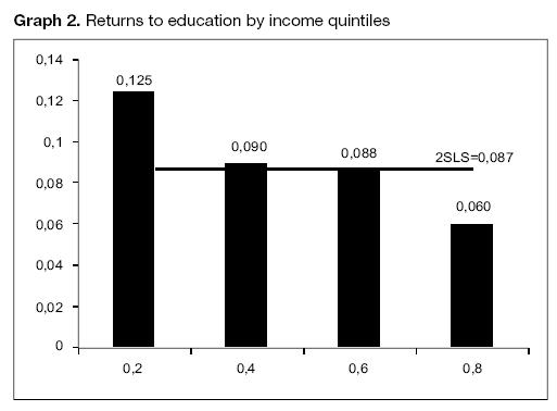
How can be explained this decreasing tendency? the results suggest that people from lower quantiles, profit more from each additional year of schooling than those belonging to the right extreme of income distribution. We may suggest that there are certain factors that increase with the income quintile such as quality of social networks, more favorable family environment, motivation, among others. This means that, at a given schooling level, richer people have more chances to get better jobs than poorer people, due to wider connections and more people belonging to their social network that occupy high quality jobs. These factors cause that people from higher quantiles obtain higher earnings independently of their schooling level, while the marginal benefit of educational investment for the poorest is greater. Having this is mind, it makes sense that the schooling coefficient for the lowest quintiles doubles the coefficient for the highest quintile.
Chernozhukov and Hansen (2005), provide an alternative explanation to the decreasing coefficient as quantile increases. They consider the quintile to which an individual belong as a proxy of his `unobserved’ ability: "people with high unobserved ‘ability’, as measured by the quantile index will generate high earnings regardless of their education level, while those with lower ‘ability’ gain more from the training provided by formal education" (p. 21). The problem of Chernozhukov and Hansen’s explanation is that it implies that ability and education are substitutes in the production of income, while it is more sensible to think that these attributes are complements: schooling fosters ability, at least when education is of reasonable quality.
The results of the other variables can be interpreted as follows (Table 3).
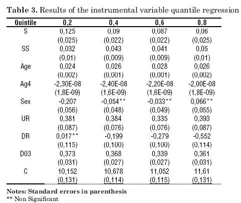
- The coefficient for spouse schooling is positive and significant for all quintiles - it slightly increases with the quantile -. It is observed that the gap between the coefficient for the head’s schooling and the spouse’s schooling is higher for the lowest quintiles: for the richest groups, the schooling of the spouse is almost as important as the head schooling in determining the income of the household, while for the poorer groups, schooling of the head is more decisive.
- The coefficient of the gender of the head is only significant for the lowest quantile, showing a marked disadvantaged of the poorest female headed households. For the other quantiles, the gender does not seem to be an important determinant of the income. This result is different when the variable spouse schooling is not included in the income equation. Table A1 in the appendix shows that, in this case, the coefficient of gender is significant and reflects a disadvantaged for the female headed households.
- Households living in urban areas tend to have more income than in rural areas. The result is consistent with the poverty measures for Colombia, according to which the inhabitants of rural areas are significantly poorer than those in urban areas: 68% of the rural population is poor, compared to 47% in urban areas.
- The coefficient corresponding to the variable ‘dependency rate’ is negative except for the lowest quantile. It makes a lot of sense that the sign of the coefficient for the poorest groups is positive, since children belonging to them start participating in the labor market at a shorter age. However, the coefficient is not significant for this quintile. We will see that, in the rural areas, the coefficient is significant and positive.
3.2. Household income by gender of the head
There are some interesting findings from the analysis by gender of the head and urban-rural location of the household3 (Tables A3 and A4 in the appendix).
Perhaps the most interesting one is that the schooling coefficient corresponding to women at rural areas is the highest compared to the coefficient of any other group (Graph 3). On the contrary, the coefficient for men at rural areas resulted non significant . There are two possible factors explaining this result. First, around 25% of male heads at rural areas work as farm-laborers, where physical abilities are more important than intellectual abilities; this proportion is 5,7% for women. Besides, only 2,3% of male heads are public servants compared to 8,3% of female heads (for the highest quantiles these proportions are 7% and 26% respectively). This job position does positively reward education. Second, education of female heads might have a higher multiplicative effect towards the rest of the family because women spend more time with their children than do men (Coleman and Ganong, 2003). Thus, an educated mother plays a more important role in determining household income than an educated father.
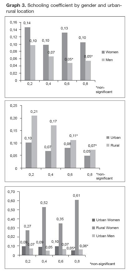
The result for rural female head of households may have important implications when designing rural educational policies. In Colombia, only the 28% of people (men and women) at schooling age in rural areas has access to media education (two last years of secondary school). According to the Ministry of education, there have been important achievements in the rural sector during the last decades related to the coverage rate at basic education, which is currently higher to 90%. However, there are little options for young people to continue studying after basic education due to the necessity of contributing to the household income. There are studies revealing that education of the mother is more important than education of the father in determining children schooling achievements: a survey conducted in 2008 by the National Council for Educational Research and Training4 said that the learning capability of children increased by 9% to 13% (7% to 11%) as the mother’s (father’s) schooling level increased from illiterate to graduation. Hence, educating female heads at rural areas brings high returns, both private and social.
Comparing the schooling coefficient by gender in urban areas and for the complete sample, we observe that education of the head has a higher impact on the income level of femaleheaded households. The result is similar to what has been found by other researchers - not for head of households but the total population - as Psacharopoulos and Patrinos (2004) on the wage return to schooling, according to which men’s return equals 8,7 while women’s equals 9,8. Again, one source of explanation for our result is the higher multiplicative effect of the female heads schooling, given the bigger amount of time that mothers spend with their children compared to fathers. Thus, the schooling spillovers should be also higher.
Another interesting result is the coefficient of the variable dependency rate in the case of rural female headed households: it shows a positive relationship between family income and dependency rate, while the coefficient is negative for urban areas and the total of households (non-significant in the case of rural male heads). This might be a reflect of the higher participation of youngsters in the labor market to support a mother head of household in rural areas.
3.3. Non-Monetary schooling returns
3.3.1. Education and health
We consider here two indicators of health:5 percentage of members of the household affiliated to the health system and average health conditions of the members of the household. Table 4 shows the results of the regressions.
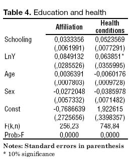
All the covariates are significant to explain the percentage of affiliation to the health insurance system. Additional years of schooling positively influence the probability of affiliation. The sources of this effect are that more education enlarges the possibilities for an individual to get a formal job, which facilitates his own affiliation and the affiliation of his family to the health system. In Colombia, having access to the health services is necessarily linked to the labour market: employees, employers, self-employed, and their dependents. Being health a fundamental human right, it is unavoidable to criticize this system in an economy with such a high levels of unemployment (12,2%, DANE, 2009). Although Colombia6 has a subsidized health regime, the coverage of this is far from universal, and the quality of the service is still an urgent issue to be tackled.
As for family health conditions, schooling level of the head is relevant in determining family health because education may help to improve habits of nutrition, smoking, alcohol consumption, sports practice, among others.7
The head’s own health is positively impacted since a better educated person has higher chances of choosing an occupation with lower risks; besides, because of his better possibilities of getting higher earnings, he may have the option to choose a better location for living. The poorest neighborhoods in developing countries have serious problems of public health due mainly to dusted streets and non treated sewage waters, which obviously affect individuals’ health. Grossman (2005) claims that schooling is the most important correlate of good health, making stronger his point noticing that "this finding emerges whether health levels are measured by mortality rates, morbidity rates, self-evaluation of health status, or physiological indicators of health, and whether the units of observation are individuals or groups" (p. 32).
3.3.2. Education and housing
We now regress an index of housing conditions on schooling of the head of the household and income, gender of the head and urban-rural location of the house. The Hausmann test of endogeneity revealed that the variables schooling and income of the household are not exogenous (the same instruments were used as before). It is observed on Table 5 that, using the proposed index and the principal component analysis (PCA), although changes the values of the coefficient, does not affect the significance or signs.
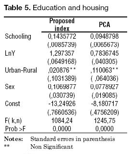
We find that differences in housing conditions are not only explained by differences in income between households, but also by the schooling level of the head. This separate effect of schooling can be explained by the fact that better-educated people have more appropriate spending priorities than less -educated people: comparing households within the same income range, housing conditions are better the higher is the educational level of the head. In addition, more educated people have a better access to the credit market, which creates the possibility to improve the conditions of the house. If we had information about permanent income, it is likely that this relationship between housing conditions and income would be more strongly perceived.
3.4. Vector of schooling returns
The returns to education of the head of households by gender (w, m) and for the poorest quintile (Q1) in Colombia are like in Equation 10, where the four elements of the set correspond to the schooling coefficient for income, affiliation to the health system, average health conditions of the family, and housing conditions respectively.8
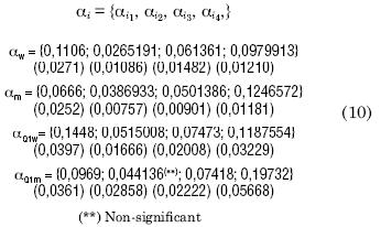
The coefficients for female heads are higher than those for male heads in the income equation, both for the 2SLS and for the lowest quintiles. This is a good signal of the great benefits that educational policies - beyond basic education - directed to these groups would bring. As for the non-pecuniary returns, all coefficients are lower for female heads except the one corresponding to health conditions. This is coherent with findings of previous research, where the role of the mother is identified as having a key role in determining lower mortality of children, higher possibilities of good nutrition of the family, higher rate of children vaccination, among other factors that will benefit family’s health.
4. CONCLUSIONS
Poverty and inequality are usually thought as problems of multidimensional nature. Likewise, returns to education should be analyzed as a multidimensional concept. In this empirical article we explore, using Colombian data, the benefits that schooling level of the head of the household brings to three poverty dimensions, namely, income, health and housing conditions.
When estimating the monetary returns, we use an instrumental variable quantile regression technique (IVQR). This is a very helpful method especially when one is interested in distinguishing the effects of an explanatory variable for the lowest or highest tails in the distribution function of the dependent variable. In fact, our estimates confirm the suspected heterogeneity of the income effect of education across quantiles of the conditional household-income distribution: the coefficient for the lowest quintile doubles the coefficient for the highest quintile.
These results suggest that people from the poorest groups profit more from each additional year of schooling than those belonging to the right extreme of income distribution. We may suggest that there are certain factors that increase with the income quintile such as quality of social networks, more favorable family environment, motivation, among others. This means that, at a given schooling level, richer people have more chances to get better jobs than poorer people, due to wider connections and more people belonging to their social network that occupy high quality jobs. These factors cause that people from higher quantiles obtain higher earnings independently of their schooling level, while the marginal benefit of educational investment for the poorest is greater.
We also made the estimations of monetary returns by gender of the head and urban-rural location of the household. We found that, for the extreme quantiles, the schooling coefficient corresponding to women at rural areas is the highest compared to the coefficient of any other group. This result for poor rural female household heads may have important implications when designing rural educational policies, especially considering that the education of the mother is more important than education of the father in determining children schooling achievements, as well as health conditions of the family. Educating women head of households at rural areas brings high returns, both private and social.
As for the non-monetary returns, we found that education of the head is significant to explain the affiliation of the family members to the health system, the average health conditions of individuals and the housing conditions. The incidence of schooling on poverty goes far beyond the income effects: higher knowledge may favorably shape individuals behaviour and influence their decisions, which will be of advantage to improve quality of life measured as satisfaction of basic needs.
We can surely continue improving the techniques to estimate returns to education, but what is most important is to keep exploring these returns as a concept of multidimensional nature. It is also relevant to think about the policy implications of recognizing the fundamental role of the heads’ education level in shaping the socioeconomic characteristics of the household they lead. In this sense, there are at least three spaces of action: the first one is directly preventing young parenthood, which might be an obstacle for the head to reach high educational achievements. A second one is widening the coverage and quality of education for adults. A third action is related to find mechanisms to counterweight the influence of parents low education on children’s outcomes, especially by separating the opportunity to reach high educational achievements from the family income level.
FOOT NOTES
1. I am grateful to the Colombian Department of Statistics (DANE) for providing the database. The support and comments of my supervisor Erik Schokkaert have been fundamental. I am also grateful to professors Paul de Grauwe and Geert Dhaene, and my colleagues Bram Thuysbaert and Julio Cesar Alonso, who gave useful comments to an earlier version of the article.
2. The results for the quantile regression, no instrumenting schooling, are shown in table A2 in the appendix. Our models were estimated by using the Matlab code developed by Chernozhukov and Hansen (2001, 2004, 2005), available on the webpage http://faculty.chicagobooth.edu/christian.hansen/research/index.htm
3. Let us recall that these results correspond to the returns to education for heads of households. The coefficient would most probably differ if we had used a broader sample, since, for instance, being a woman head of household is not a random characteristic.
4. National Council of Educational Research. Educational Survey. http://www.ncert.nic.in/html/educationalsurvay.htm
5. In Colombia, the health system has two different regimes: contributive and subsidized. The fi rst one is jointly paid by workers (1/3) and employers (2/3), or by independent workers. An affiliated worker can enroll his/her children and partner. The second system is directed to people with no capacity to pay. The total coverage is only 74% (33,7% contributive and 40,4% subsidized from www.minproteccionsocial.gov.co). There are public and private suppliers of both regimes.
6. Information provided in: www.dane.gov.co
7. There is also empirical evidence revealing higher rate of vaccinations among children of better educated parents (Haveman and Wolfe, 1984).
8. Standard deviations in parenthesis.
BIBLIOGRAPHIC REFERENCES
1. Angrist, J. and Krueger. A. (1991). Does compulsory schooling attendance affect schooling and earnings? Quarterly Journal of Economics, 106(4), 979-1014. [ Links ]
2. Angrist, J. and Krueger. A. (1992). Estimating the payoff to schooling using the Vietnam-Era draft lottery (NBER Working Paper No. 4067). Available at: http://www.nber.org/papers/w4067 [ Links ]
3. Ashenfelter, O. and Krueger, A. (1994). Estimates of the economic return to schooling from a new sample of twins. American Economic Review, 84, 1157 - 1173. [ Links ]
4. Atkinson, A.B. and Bourguignon, F. (1982). The comparison of Economics Multi-dimensioned distribution of Economics Status. Review of Economics Studies, 49, 183-201. [ Links ]
5. Becker, G. (1965). A theory of the allocation of time. Economic Journal, 75, 493-517. [ Links ]
6. Becker, G. (1993). Human Capital. New York, NY: Columbia University Press. [ Links ]
7. Becker, G. and Lewis, G. (1973). On the interaction between quantity and quality of children. Journal of Political Economy, 81, 279-288. [ Links ]
8. Borooah, B. (2002). Logit and Probit: ordered and multinomial models. Thousand Oaks, CA: Sage. [ Links ]
9. Bourguignon, F. and Chakravarty, S. (1999). A family of multidimensional poverty measures. In D. Slottje (Ed.), Advances in econometrics Income Distribution and Scientific Methodology (pp. 331- 344). Heildelberg, NY: Physica- Verlag. [ Links ]
10. Bourguignon, F. and Chakravarty, S. (2003). The measurement of multidimensional poverty. Journal of Economic Inequality, 1, 25-49 [ Links ]
11. Card, D. (1993). Using Geographic Variation in College Proximity to Estimate the Return to Schooling (NBER Working Paper No. 4483). Available at: http://www.nber.org/papers/w4483 [ Links ]
12. Chernozhukov, V. and Hansen, C. (2001). An IV model of Quantile Treatment Effects (Working paper MIT). Available at: http://www.mit.edu/~vchern/papers/ch_iqr_ema.pdf [ Links ]
13. Chernozhukov, V. and Hansen, C. (2004). Instrumental variable quantile regression (Working paper MIT). Available at: http://www.mit.edu/~vchern/papers/ch_IVQR_2001_rev_Oct24_2004.pdf [ Links ]
14. Chernozhukov, V. and Hansen, C. (2005). Instrumental quantile regression inference for structural and treatment effect models. Journal of Econometrics, 132, 491- 525. [ Links ]
15. Cheser, A. (2005). Instrumental values. London: Centre for Microdata Methods and Practice, Institute for Fiscal Studies and University of London. [ Links ]
16. Coleman, M. and Ganong, L. (Eds). (2003). Handbook of contemporary families. Thousand Oaks, CA: Sage. [ Links ]
17. Ettner, S. (1996). New evidence on the relationship between income and health. Journal of Health Economics, 15, 67-85. [ Links ]
18. Foster, J., Greer, J. and Thorbecke, E. (1984). Notes and comments a class of decomposable poverty measures. Econometrica, 52, 761- 766. [ Links ]
19. González, N., Gómez, J., Mora, J. and Zuluaga, B. (2004). Las ganancias de señalizar en el mercado laboral en Cali. Estudios Gerenciales, 92, 105-128. Available at: http://biblioteca2.icesi.edu.co/cgi-olib?session=88586072&infile=&sobj=1426&source=webvd&cgimime=application%2Fpdf [ Links ]
20. Grossman, M. (2005). Education and non-market outcomes (NBER Working Paper No. 11582). Available at: http://www.nber.org/papers/w11582.pdf [ Links ]
21. Harmon, C. and Walker, I. (1995). Estimates for the economic return to schooling for UK. American Economic Review, 85, 1278-1286. [ Links ]
22. Haveman, R. and Wolfe, B. (1984). Schooling and economic well-Being: The role of non-market effects. Journal of Human Resources, 19, 378-407. [ Links ]
23. Hungerford, T. and Solon, G. (1987). Sheepskin Effects in the Returns to Education. Review of Economics and Statistics, 69, 175- 177. [ Links ]
24. Kenkel, D. (1991). Health Behavior, Health Knowledge, and Schooling. Journal of Political Economy, 99(2), 287–305. [ Links ]
25. Koenker, R. (2005). Quantile Regressions. Cambridge: Cambridge University Press. [ Links ]
26. Koenker, R. and Bassett, G. (1978) Regression Quantiles. Econometrica, 46, 33-50. [ Links ]
27. Koenker, R. and Hallock, K. (2001). Quantile Regression. Journal of Economic Perspectives, 15, 143- 156. [ Links ]
28. Layard, R. and Psacharopoulos, G. (1974). The Screening Hypothesis and the Returns to Education. Journal of Political Economy, 82, 985-998. [ Links ]
29. Lemieux, T. (2006). The "Mincer Equation" Thirty Years after Schooling, Experience, and Earnings. In: J. Mincer (Ed.), A Pioneer of Modern Labor Economics (chapter 11). New York, NY: Springer US Editor. [ Links ]
30. Michael, R. (1972). The Effect of Education on Efficiency in Consumption. New York, NY: Columbia University Press for the NBER. [ Links ]
31. Michael, R.T. and Willis, R. (1976). Contraception and Fertility: Household Production under Uncertainty. In N.E. Terleckyj (Ed.), Household Production and Consumption Studies in Income and Wealth (pp. 25-98), 40. [ Links ]
32. Mincer, J. (1974). Schooling Experience and Earnings. New York, NY: Columbia University Press for the National Bureau of Economic Research. [ Links ]
33. Psacharopoulos, G. and Patrinos, H. (2004). Returns to investment in education: a further update. Education Economics, 12, 111- 134. [ Links ]
34. Rodríguez, J. and Ramírez, C. (2002). Pobreza en Colombia: tipo de medición y evaluación de políticas en los años 1950 y 2000. Estudios Gerenciales, 85, 81-107. Available at: http://biblioteca2.icesi.edu.co/cgi-olib?session=42018015&infi le=&sobj=532&source=webvd&cgimime=application%2Fpdf [ Links ]
35. Schultz, T. (1961). Investment in Human Capital. American Economic Review, 51, 1-17. [ Links ]
36. Schultz, T. (1973). The value of children: an economic perspective. Journal of Political Economy, 81, 2-13. [ Links ]
37. Sen, A. (1976). Poverty: An ordinal approach to measurement. Econometrica, 44, 219-231. [ Links ]
38. Sen, A. (1985). Commodities and capabilities. Amsterdam: North- Holland. [ Links ]
39. Sen, A. (1999). Development as Freedom. New York, NY: Knopf. [ Links ]
40. Strauss, J. (1990). Households, Communities, and Preschool Childrens Nutrition Outcomes: [Evidence from Rural Côte dÎvoire. Economic Development and Cultural Change, 38(2), 231-261. [ Links ]
41. Trostel, P., Walker, I. and Woolley, P. (2002). Estimates of the economic return to schooling for 28 countries. Labour Economics, 9, 1-16. [ Links ]
42. Tsui, K.Y. (1994). Multidimensional poverty Indices. Hong Kong: Chinese University of Hong Kong. [ Links ]
43. Tsui, K.Y. (2002). Multidimensional poverty indices. Social Choice and Welfare, 19(1), 69-94. [ Links ]
44. Verbeek, M. (2000). A guide to modern econometrics. West Sussex, England: John Wiley & Sons. [ Links ]
45. Williams, D. (2002). Returns to education and experience in self-employment: evidence from Germany (IRISS Working Paper No. 2002-04 CEPS/INSTEAD). Available at: http://iriss.ceps.lu/documents/irisswp27.pdf [ Links ]
46. Willis, R. (1973). A new approach to the Economic theory of fertility behaviour. Journal of Political Economy, 81, 14-64. [ Links ]
47. Wooldridge, J. (2002). Econometric Analysis of Cross Section and Panel Data. London: The IMT Press. [ Links ]
48. Zuluaga, B. and Bonilla, D. (2005). El papel de las Instituciones educativas públicas en la reducción de la pobreza. Estudios Gerenciales, 97, 31-59. Available at: http://biblioteca2.icesi.edu.co/cgi-olib?session=25929564&infi le=&sobj=2101&ource=webvd&cgimime=application%2Fpdf [ Links ]

