


 Inglés (pdf)
 Articulo en XML
 Referencias del artículo
 Enviar articulo por email
 Citado por SciELO
  Citado por Google
  Similares en
SciELO
Similares en
SciELO  Similares en Google
 Permalink
1. Introduction
Decisions about whether to grant credit or not play a crucial role in lending institutions. Insight into factors leading to business failure and solvency indications can make the difference between profit or loss. Both studies on significant economic-financial indicators for credit analysis or on methodologies to help provide credit are economically and socially important.
Managers must take into consideration the risks involved when there is a high volume of credit operations. At present, risks concern constant costs in credit operations; therefore, they are worth quantifying. The idea of risk is associated with the likelihood of facing outcomes related to expected returns; thus, risk heads towards the future and points out possible losses (Assaf Neto, 2014). Financial operations involving credit must be protected against constant operational risks or, at least, turn uncertainty into measurable risks (Silva, 1983).
The first publications in this field were an attempt to detect whether indicators of solvent companies were favorable and whether the indicators of insolvent companies were unfavorable. Some of the main (univariate) studies conducted in this field were The Use of Multiple Measurements in Taxonomic Problems by Fisher (1936) and Risk Elements in Consumer Installment Lending by Durand (1941). The univa- riate analyses performed in the late 1950s were replaced as soon as scholars turned their attention to credit scoring modeling techniques in the late 1960s (Sabato, 2009).
Seminal studies in this field were Financial Ratios as Predictors of Failure by Beaver (1966) and Financial Ratios, Discriminant Analysis and the Prediction of Corporate Bankruptcy by Altman (1968). These two studies mark the beginning of research based on multivariate discriminant analysis, which became a common technique in research on the topic until a publication by Ohlson (1980) called Financial Ratios and the Probabilistic Prediction of Bankruptcy. He applied the logit model to forecast bad debt, opening up the possibility of using other methodologies in this research field. A decade later, Odom and Sharda (1990) suggested a new model in their study A Neural Network Model for Bankruptcy Prediction, which was based on artificial intelligence techniques known as artificial neural networks.
Nowadays, there are many tools capable of carrying out credit analysis. Multivariate analysis techniques such as discriminant analysis and logistic regression are the most traditional tools to build credit risk models. Kumar and Ravi (2007) and do Prado et al. (2016) suggest that the 1990s brought along significant changes in this field, since publications based on logistic regression and neural networks became more numerous than the ones based on discriminant analysis, although it ‘‘was a very popular method for model development in the early stages of bankruptcy prediction’’ (Bellovary, Giacomino, & Akers, 2007, p. 2). However, Computational Intelligence techniques have called the attention of researchers to new possibilities (Barboza, Kimura, & Altman, 2017; Liu & Wu, 2019; Pal, Kupka, Aneja, & Militky, 2016; Santana, Lanzarini, & Bariviera, 2018; do Prado et al., 2016).
Kumar and Ravi (2007) and Wang, Ma and Yang (2014) state that literature in the financial field does not address the most expressive indicators in insolvency assessments. According to them, indicators are often chosen when they are related to data access and to researchers’ perspectives, although different indicators are systematically applied in different studies.
Accordingly, the aims of this research are to identify the economic-financial indicators that best contribute to improving the accuracy of credit granting analyses applied to Brazilian public companies, and to assess the most accurate techniques (discriminant analysis, logistic regression and artificial neural networks) used in business bankruptcy forecasting.
Barboza et al. (2017) and do Prado et al. (2016) point out that credit risk analyses have been the subject of a series of in-depth studies in recent years. They are the main focus of financial and banking fields, mainly because of the recent international financial crisis, which had a severe effect on many financial organizations. Enhanced methodologies and the evolution of forecasting techniques help managers to keep business liquidity organized, since these techniques help to avoid bad debt or even bankruptcy. Bankruptcy leads to major problems in the market since it regards capital losses and social damages.
Studies on company solvency are relevant because they reinforce research into finances, provided there is good understanding about company behavior and financial strategies. The goal of the present approach is to help broaden knowledge of theoretical and empirical analyses applied to credit risks and of their potential to be used in business decision enhancement within the Brazilian capital market.
The present study addresses a theoretical framework of credit, its risks and the analysis thereof. The methodology highlights the main credit analysis indicators. Results of the credit analysis approach (discriminant analysis, logistic regression, artificial neural networks) were presented and individual analysis was applied to relevant financial indicators.
2. Theoretical framework
Soares and Rebouças (2015, p. 41) highlight that “supporting credit risk reduction is one of the most popular applications of solvency forecasting”. Credit plays an important economic and social role in companies’ lives. Silva (2008) stated that credit must enable companies to intensify their activities, encourage consumption and increase demand, as well as to fund projects that cannot be run only with internal resources. However, the inadequate use of credit can lead to bankruptcy (insolvency).
Uncertainty is a variable inherent to credit granting that is ever-present. According to Sicsú (2010), financial institutions are always subjected to the likelihood of loss in this type of transaction; thus, it is recommended to quantify loss probabilities in order to better classify appropriate loan applicants. According to the aforementioned author, “loss probabilities in credit operations are called credit risks” (Sicsú, 2010, p. 1).
Based on Silva (2008), multivariate statistical techniques are powerful tools to manage existing bad-debt risks in the provision of credit. The most efficient statistical technique to model companies’ data must be identified in order to better forecast clients’ behavior and to generate a credit risk forecasting model.
Schrickel (2000) states that credit is somehow connected to the likelihood of losses because it involves expectations about the return of the granted property. García, Guijarro and Moya (2013) and Yu (2014) emphasize that credit risk analyses have been the target of a series of detailed studies conducted in recent years. Credit risk became the main focus of both financial fields and banks, given the international financial crisis, which had a serious effect on many financial organizations. Bülbül, Hakenes and Lambert (2019) and Oreski and Oreski (2014) note that credit risk management, which has been significantly enhanced in recent decades, is one of the most important issues for the banking sector.
Assaf Neto (2014) states that risk is a cost often found in business; therefore, it must be quantified. García et al. (2013) argues that credit risk management is a key issue for companies at any time. The aforementioned authors also highlight several current methodologies aimed at forecasting bad-debt probabilities involving debtors. Some of these methodologies use logit analysis, or discriminant analysis, to classify debtors; however, new methodologies use neural networks or multi-criteria methods.
Based on Harris (2013), competition increase in the financial service sector helped companies to find innovative ways to deal with risk in order toreach and/or keep competitive advantages. Financial institutions face a greater risk of losses associated with inadequate credit approval, often due to poor decision-making in the context of the economic environment and current business. However, Kou and Wu (2014) state that the main goal of credit risk analysis lies in classifying clients as good or bad payers (solvent or insolvent).
According to Sicsú (2010), credit risk quantification through quantitative analysis techniques is a great advantage, since these techniques are faster, more consistent and lead to more adequate decisions. In addition, Kimura, Suen, Perera and Basso (2008) state that risk management through research and quantitative model implementations are becoming increasingly common in modern businesses.
Silva (2008) highlights that quantitative methods have been widely disseminated, making banks seek these techniques to assess credit risk. However, these forecasting methods cannot be interpreted as a ‘magic bullet’ to solve all issues linked to credit risks in financial operations.
3. Methodology
The present study can be classified by ends, means, data type and approach. The study is predominantly explanatory (Vergara, 2008) and its means can be categorized as ex post facto (Vergara, 2008). A literature review and document search were used for secondary data (Marconi & Lakatos, 2005). The document search was conducted in the annual financial reports available on the Economática®database, and at the website of BM&FBOVESPA (Stock, Commodities and Future Market). The research follows the quantitative approach (Martins & Theóphilo, 2009). SPSS (Statistical Package for Social Sciences) and Minitab software were used to develop the study.
Insolvency is defined in the Bankruptcy and Concordat Law n. 7661, from June 21st 1945 (Brasil, 1945), which was repealed by Law n. 11101, from February 2005 (Brasil, 2005). At present, this law covers all current bankruptcy and concordat cases, meaning that the event determining companies’ bankruptcy filing will be the time when they issue the formal Preventive Bankruptcy Filing or the Judicial Recovery at the Securities Committee (CVM - Comissão de Valores Mobiliários).
The year before companies had issued the bankruptcy filing (the year before the event, timet-1) provided their insolvency indicators. However, whenever possible at least one solvent company was selected for each insolvent company from the same economic sector, with accounting assets proportional to those of the insolvent institution. This methodology is based on previous studies by Altman (1968), Brito, Assaf Neto and Corrar (2009), and Sanvicente and Minardi (1998).
The number of insolvent companies was selected to enable sample size analyses, so that the modeling processes applied to the approached techniques would not be impaired. The sample comprised 121 companies; 70 solvent and 51 insol- vent. The sample size used followed the recommendations by Hair et al. (2009, p. 236), who state that there must be at least 40 companies from each of the previously defined groups.
3.1 Defining the indicators
The most common indicators in studies in this field were used to select Traditional Financial Analysis Model indica- tors, which were defined based on considerations by Pereira, Domínguez and Ocejo (2007). They state that empirical evidence points out that new studies tend to choose indicators from previous studies that have recorded satisfactory results. Table 1 presents the indicators selected for the financial analysis, given their compliance with the selected theoretical reference and with the scope of the present research.
Table 1 Economic-financial indicators.
| Code | Indicators | Formula | Authors |
|---|---|---|---|
| X1 | WC on assets | WC / TA | Presented in the current study based on studies by Fleuriet et al. (2003) |
| X2 | WC on net income | WC / NI | |
| X3 | NWC on assets | NWC / TA | Brito, Assaf Neto and Corrar (2009) and Minussi, Damacena and Ness Junior (2002) |
| X4 | NWC on net income | NWC / NI | |
| X5 | Balance in treasury on assets | BT / TA | Brito, Assaf Neto and Corrar (2009), Horta (2010) and Sanvicente and Minardi (1998) |
| X6 | Balance in treasury on net income | BT / NI | |
| X7 | Financial liabilities over Current assets | FL / CA | Eifert (2003) |
| X8 | Financial Structure Type | FST | Melo and Coutinho (2007) |
| X9 | Liquidity Thermometer - LT | BT / (|NWC|) | Horta (2010) and Vieira (2008) |
| X10 | Balance in treasury | BT= FA - FL | Melo and Coutinho (2007) |
| X11 | Need of working capital | NWC = OA - OL | Melo and Coutinho (2007) |
| X12 | Working Capital | WC = NCL - NCA | Melo and Coutinho (2007) |
| X13 | Indebtedness | (FL + NCFL) / TA | Brito, Assaf Neto and Corrar (2009) |
| X14 | Net working capital | (CA - CL) / TA | Altman (1968), Brito, Assaf Neto and Corrar (2009), and Sanvicente and Minardi (1998) |
| X15 | Return on assets | EBIT / TA | Altman (1968), Altman, Baydia and Dias (1979) and Brito, Assaf Neto and Corrar (2009) |
| X16 | Shareholder’s equity divided by the total liabilities | NE / TL | Altman, Baydia and Dias (1979), Horta (2010) and Soares and Rebouças (2015) |
| X17 | Asset turnover | NI / TA | Altman (1968), Brito, Assaf Neto and Corrar (2009) and Castro Junior (2003) |
| X18 | Return on Assets | NP / TA | Eifert (2003), Horta (2010) and Soares and Rebouças (2015) |
| X19 | Retaining earnings on assets | (AP + NI) / TA | Brito, Assaf Neto and Corrar (2009) |
| X20 | Shareholder’s equity return | NP / NE | Castro Junior (2003), Brito, Assaf Neto and Corrar (2009) and Kanitz (1978) |
| X21 | Current Liquidity | Castro Junior (2003), Horta (2010), Matias (1978) and Silva (1983) | |
| X22 | Liquidity dry-ups | CA / CL (CA - stocks) / CL | Brito, Assaf Neto and Corrar (2009) e Horta (2010) and Kanitz (1978) |
| X23 | General liquidity | (CA + RLT) / (CL + NCL) | Kanitz (1978) and Soares and Rebouças (2015) |
| X24 | Operating income on financial expenses | EBIT / FE | Brito, Assaf Neto and Corrar (2009) and Soares and Rebouças (2015) |
| X25 | Net margin | NP / NI | Brito, Assaf Neto and Corrar (2009) and Castro Junior (2003) |
| X26 | Total Debt | (CL + NCL) / TA | Brito, Assaf Neto and Corrar (2009), Horta (2010) and Silva (1983) |
| X27 | Structure indicator | SUPLIER / TA | Matias (1978) and Silva (1983) |
| X28 | Debt breakdown | CL / (CL + NCL) | Castro Junior (2003) |
| X29 | Third capital participation | (CL + NCL) / NE | Castro Junior (2003) |
| X30 | Immobilization of equity | FIXED ASSETS / NE | Brito, Assaf Neto and Corrar (2009), Castro Junior (2003) and Soares and Rebouças (2015) |
| X31 | Equity on assets | NE / TA | Brito, Assaf Neto and Corrar (2009) and Matias (1978) |
| X32 | Stocks on assets | STOCKS / TA | Brito, Assaf Neto and Corrar (2009), and Silva (1983) |
| X33 | Immediate liquidity | AVAILABLE / CL | Brito, Assaf Neto and Corrar (2009), Castro Junior (2003) and Horta (2010) |
| X34 | Structure indicator | AVAILABLE / TA | Matias (1978), Silva (1983) |
| X35 | Structure indicator | AVAILABLE / NCA | Silva (1983) and Soares and Rebouças (2015) |
CA = Current assets; NWC = Need of working capital; FA = Financial assets; CL = Current liabilities; OA = Operating asset; FL = Financial liabilities; NCA = Non-current assets; NE = Net equity; TA = Total assets; OL = Operating liabilities; WC = Working capital; NCL = Non-current liabilities; FE = Financial expenses; NCFL = Non-current financial liabilities; FST = Financial Structure Type; = RLT = Realizable in the long term; TL = Total liabilities ; BT = Balance in treasury; AP = Accumulated profits; LT = Liquidity thermometer; EBIT = Earnings before interests and income taxes; NI = Net income; NP = Net profit
Source: own elaboration
According to Bellovary et al. (2007), the number of indicators used in models has been analyzed through decades and these analyses show that the mean values have varied throughout time, while remaining close to 10 indicators on average. Techniques such as stepwise were recommended to help eliminate less significant indicators (based on F statistics) in order to conduct more parsimonious models and to identify the main economic-financial indicators that best distinguish solvent from insolvent companies in credit granting analysis.
Models were created after sampling data (solvent and insolvent companies) were collected. Data were subjected to the respective analyses and comparisons. Discriminant analysis (Hair et al., 2009), logistic regression (Hosmer & Lemeshow, 2004) and neural network models (Haykin, 2007) were used in the current study. Some practical examples of these methodologies can be seen in studies by Castro Junior (2003), Iturriaga and Sanz (2015), and Soares and Rebouças (2015).
4. Results and discussion
Three methods for indicator combinations were tested for model creation: 1) result of stepped methods, 2) result of advanced methods and, 3) human trial and error process. Thus, several possible combinations of indicators were tested for each model. The best results found for each model are presented in the next topics.
4.1. Discriminant analysis (DA)
The best model for discriminant analysis was found through a process of trial and error. The significant indicators (sig. < 0.05) were the relevant parameters for the modeling. The canonical correlation (0.814)2 explained the 66% discrimination between groups. There was no stronger multicollinearity correlation (tolerance value > 0.1 and VIF values <10).
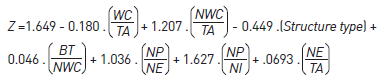
The classification function coefficient analysis shows a little more about the importance of each indicator in the discrimi-nant function. Indicators presenting negative discriminant function coefficient values were Working Capital on Assets (X1- WC / TA) and Financial Structure Types (X8- FST = Financial Structure Types). These indicators helped to classify compa-nies as insolvent. On the other hand, indicators presenting positive discriminant function coefficient values were Need of Working Capital on Assets (X3- NWC / TA); Liquidity Thermometer (X9- LT = BT / (|NWC|)); Shareholders’ Equity Return (X20- NP / NE); Liquid Margin (X25- NP / NI); and Net Equity on Assets (X31- NE / TA). These helped classify companies as solvent.
As soon as the non-standardized canonical discriminant function coefficients were found, it was possible to elaborate the Discriminant Analysis function, i.e., the generated credit scoring could be expressed in equation 1:
 (1)
(1)
After elaborating the Discriminant Analysis Function, the cut-off point was calculated based on the centroids in each group, which were the means found through the individual distribution of groups. The weighted average between centroids in each one of the distributions set the cut-off point of the discriminant function. The optimal cut-off point recorded was 0.4978, this value classifies companies through their discriminant score, i.e., companies recorded below -0.4978 belonged to group “1” (insolvent) and companies recording discriminant scores above this belonged to group “0” (solvent).
4.2. Logistic regression (LR)
The Forward: LR method was applied to calculate the Logistics Regression, which recorded the best results. We validated the results through the following parameters:
Cox & Snell 59%; Nagelkerke 79%; and Log-likelihood -2 (-2VL) 64.5% to explain the reasons why companies become insolvent; Hosmer and Lemeshow Sig. > 0.05 and Multicollinearity (Tolerance values > 0.1 and VIF values <10).
Results of indicators in the model presented the positive aspects of the attempts to estimate probabilities based on each coefficient. The Wald statistics presented a Wald coefficient higher than zero (wald >0) in each of the factors; thus, it imposed a discriminant effect over the probability of companies to be insolvent or solvent. Indicators were also significant at a probability level of 0.05 (Sig. < 0.05). Coefficients of independent factors listed in column Exp(B) (25.34) were within the limit set by the Inferior and Superior columns (3.12 to 205.38, respectively), as well as of all other used factors.
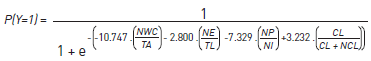
The Logistic Regression Model able to classify companies as insolvent and solvent used the regression coefficients. The Logistic Regression Equation, or the generated Credit Scoring, can be represented by Equation 2.
 (2)
(2)
P (Y =1) presented dichotomic-type output in the Logistic Regression analysis when only two possible values were taken into account, ‘0’ and ‘1’. Thus, the closer to 1, the more insolvent the company, and the closer to zero (0), the more solvent the company. The cut-off point in the Logistic Regression is 0.5, as results vary from ‘0’ to ‘1’. It is also possible to multiply this result by 100 and interpret it as the probability (in %) that a company will be insolvent.
Coefficients generated through Logistic Regression represent the influence of estimates of each independent variable (indicator) on the dependent variable (when the other indicators remain unchanged), i.e., the signal (+ or -) will set the direction (solvent = 0, insolvent = 1) to be taken by the dependent variable (solvent/insolvent). The higher the negative coefficient values, the greater the company’s possibility of being solvent (Group 0), and the higher the positive coefficient values, the greater the chance of the company belonging to the insolvent group (Group 1).
4.3. Artificial neural networks (ANN)
The best Artificial Neural Network model was found through trial and error. The Multilayer Perceptron (MLPS) network was used with feedforward architecture; a back-propagation algorithm with a training error criterion of 0.0001 was used in the modeling process. Network information is shown in Table 2. The co-variables (eight units) represented the selected indicators. The hidden layer was defined with seven neurons (units). The hyperbolic tangent was the activation function in each hidden layer; the Softmax activation function was used in the output layer. The activation functions were defined because they presented the best performance among the tested functions.
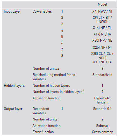
The most important indicators for the neural networks model (in order of importance) were Liquidity Thermometer (X09- LT = BT / (|NWC|)); Need of Working Capital on Net Revenue (X03- NWC / NI); Net Equity on Assets (X31- NE / TA); Shareholders’ Equity Return (X20- NP / NE); Net Margin (X25 - NP / NI); Asset Turnover (X17- NI / TA); Net Equity on Total Liabilities (X16- NE / TL) and Debt Breakdown (X28- CL / (CL + NCL)).
However, the importance of an independent indicator was calculated based on the variation faced by the network in its forecasted value (output) and in different input values. It is not possible to state that higher values of indicator ‘x’ indicate a greater probability of companies becoming insolvent.
4.4. Model comparison
Table 3 shows the accuracy of the selected models with regard to Type I and Type II Precision levels. Type I Precision was opposite to Type I Error, i.e., the higher the Type I Precision, the lower the Type I Error - the same occurs with Type II Precision.
Table 3 Accuracy recorded by means of the three final models (at Type I and II error levels)
| Model1 | Type I precision | Type II precision | General precision |
|---|---|---|---|
| Discriminant analysis2 | 82.4% | 97.1% | 90.9% |
| Logistic analysis | 90.2% | 91.4% | 90.9% |
| Artificial neural networks³ | 98.0% | 98.6% | 97.8% |
¹ The simple arithmetic means was used in the models between the re sult of the training sample and the result of the validation sample (test).
² Model error was checked through the hold-out method (Train: 90%, Test: 10%).
³ Model error was checked through the hold-out method (Train: 75%, Test: 25%).
Source: own elaboration.
The Type I and II Error level analyses performed through precision models were essential for better understanding their quality. Based on Table 3, discriminant analysis and regression logistics recorded a 90% success level. However, the results of Type I and II Precision levels show that the lo-gistic regression model is the best to classify Type I Precision, i.e., the percentage of companies classified either as insolvent or solvent is higher in the discriminant analysis model than in the logistic regression, a fact that leads to capital losses.
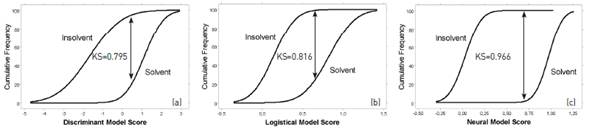
Models could also be assessed through Kolmogorov- Smirnov (KS) statistics in order to verify the score behavior of the two samples in each model. Distribution values of the generated models could improve understanding of the test by generating graphics showing the separation degree between solvent and insolvent companies through model scores (Figure 1).
Source: own elaboration.
Figure 1 Distribution of cumulative frequencies for KS in the constructed models (a = Discriminant Analysis; b = Logistic Regression and c = Neural Networks).
Models recorded values above 0.75; however, neural network superiority became evident at 0.966. This outcome was followed by the Logistic Regression (0.816) and by the Discriminant Analysis results (0.795).
Besides the KS test, authors such as Baesens et al. (2003) and Sicsú (2010) assess the discriminant power of the classification models through the analysis used to apply ROC curve values (Receiver Operating Characteristic Curves), which led to good credit risk results. Figure 2 shows the ROC curves found in the best three generated models. The discriminant analysis presented the smallest area below the curve and the logistic regression presented better results than the discriminant analysis. However, the best performance was presented by neural networks, which occupied almost all the ROC curve area.
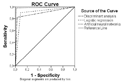
Models could be classified based on values found in the ROC curve area such as roc<= 0.5 non-exiting; 0.5<roc< 0.7 = low; 0.7<=roc<0.8 = acceptable; 0.8<=roc<0.9 = excellent; and roc>= 0.9 = above the average. Table 4 classified the discriminant analysis model below the ROC curve area in 0.897, which is an excellent outcome. On the other hand, the logistic regression and neural network models recorded 0.908 and 0.983, respectively. Both models exceeded the classification expectations, because they recorded more than excellent results.
Table 4 Values found in the ROC curve área.
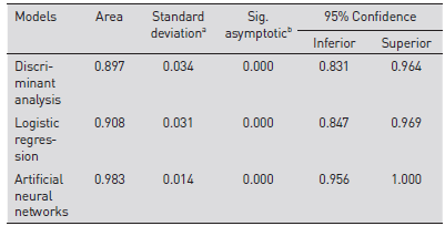
The variable, or variables, of the test results: Discriminant Analysis, Logistic Regression, Artificial Neural Networks have at least one bond between the real positive state group and the real negative state group. The statistics can be biased.
a. Under the non-parametric assumption. b. Null hypothesis: real area = 0.5.
Source: own elaboration.
Table 5 summarizes the performance measurements (Accuracy Level, Type I Error, KS tests and ROC Curve) used to compare the fine models. The Artificial Neural Networks recorded the best results in all conducted tests, i.e., high accuracy level, low Type I error, high values in the KS test and in the ROC curve.
Table 5 Performance measures in the generated models
| Models | Accuracy level | Type I error | KS Test | ROC curve |
|---|---|---|---|---|
| Discriminant Analysis | 90.9 | 17.6% | 0.795 | 0.897 |
| Logistic Regression | 90.9 | 9.8% | 0.816 | 0.908 |
| Artificial neural networks | 97.8 | 2% | 0.966 | 0.983 |
Source: own elaboration.
The classification showed correctly classified companies and companies whose models were not able to be properly classified. Only Tecnosolo, which was originally classified as insolvent, was classified as solvent based on the three models, i.e., the rules created for this company were not able to find insolvency symptoms.
4.5. Indicator analysis
Table 6 depicts the most representative indicators in all groupings; all indicator groupings used in the present study recorded precision higher than 86%. Indicators of the Fleuriet Model were found in all groupings. Forward: LR in the logistic regression, Trial and error in the discriminant analysis and Trial and error in all artificial neural networks (such as the discriminant indicators ‘X’ - in bold - in Table 6) were the final three models presenting the best results - indicators that appeared three times or more were highlighted.
Table 6 Selected Indicators
| Indicators | For-ward: LR | Step-wise | Trial and error, AD | Trial and error, ANN | Trial and error, other | Trial and error, other | Total of repetitions |
| X1) WC / TA | X | 1 | |||||
| X3) NWC / TA | X | X | 2 | ||||
| X4) NWC / NI | X | X | X | X | 4 | ||
| X8) FST = Structure | X | X | 2 | ||||
| X9) LT = BT / (|NWC|) | X | X | X | 3 | |||
| X10) BT = FA - FL | X | X | 2 | ||||
| X11) NWC = OA - OL | X | 1 | |||||
| X16) NE / TL | X | X | 2 | ||||
| X17) NI / TA | X | X | 2 | ||||
| X18) NP / TA | X | X | 2 | ||||
| X20) NP / NE | X | X | X | 3 | |||
| X25) NP / NI | X | X | X | X | 4 | ||
| X28) CL / (CL + NCL) | X | X | X | 3 | |||
| X29) (CL + NCL) / NE | X | 1 | |||||
| X30) Fixed asset / NE | X | 1 | |||||
| X31) NE / TA | X | XX | 3 | ||||
| X34) Available / TA | XX | 2 |
Source: own elaboration.
Need of Working Capital on Assets (X3); Liquidity Thermometer (X9); Shareholders’ Equity Return (X20); Net Margin (X25) and Net Equity on Assets (X31) were the selected indicators in the three final models presenting low values for insolvent companies and high values for solvent companies. On the other hand, only two indicators recorded higher values for insolvent companies, namely: Working Capital on Assets (X1) and Financial Structure Type (X8).
Of the 35 initially selected indicators, only 17 participated in the last groupings. Of all 17 indicators presented in the Table 6, indicators X18, X29, X30 and X34 were not explored.
4.5.1. Analysis of working capital on assets
The indicator Working Capital on Assets (WCA) was representative in the final model, which was generated through discriminant analysis only. The sample presented positive values for solvent companies (0.166) and negative values for the insolvent ones (-0.302) at a total average of -0.031. However, the discriminant analysis presented a negative signal (-) in the coefficient, which means that the higher the value presented by the WCA indicator, the greater the probability of a company being insolvent in the discriminant function.
This result was the only sign of divergence presented by the models. Olinquevitch and Santi Filho (2009, p. 85) state that “in analytical terms, the simple availability of WC is not enough to indicate good economic-financial health: the resources available must fit the needs”.
4.5.2. Considerations for need of working capital
According to Olinquevitch and Santi Filho (2009, p. 13), the Need of Working Capital value (NWC) can be positive or negative; a positive NWC signal indicates that Working Capital (WC) is more applicable than the WC sources, thus “expressing that the company is investing resources in the working capital”. However, when NWC is negative, WC sources are greater than applications in WC, thus “expressing that the company is profiting (getting financed) due to resources resulting from working capital” (Olinquevitch & Santi Filho, 2009, p. 13).
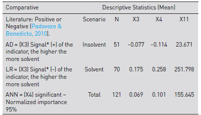
NWC on Net income and on Assets as a group was the only indicator found in all proposed groupings (Table 6). Solvent companies were positive, on average, whereas the most insolvent companies showed negative values (Table 7). This outcome was confirmed by the discriminant analysis and logistic regression models, whose values indicated that the higher the NWC value, the greater the probability of the company being solvent. This indicator was significant at 95% probability and it explained the variation in the forecasted value of the neural network (output).
Table 7 Performance measures in the generated models
*Signals presented by the discriminant analysis and logistic r9egression were opposite due to the way the calculation was performed; however, when they were inverted, they presented the same trend for the indicator: (AD = ‘+’ and LR = ‘-’); the higher the indicator, the more solvent the company.
Source: own elaboration.
These results diverge from those recorded by Minussi, Damacena and Ness Junior (2002, p. 122) who, by studying companies from the industrial sector, found NWC values on net income (IOG/net sales - variable X2”). They recorded a mean value of 0.80 for the group of solvent companies and 3.50 for the insolvent group.
Results diverging from those of Minussi et al. (2002) concerned the fact that only 4 solvent companies in the sample had Type I Financial Structure ‘Excellent’, i.e., they presented positive WC and BT, and negative NWC (Table 8). On the other hand, most solvent companies presented a ‘solid’ Type 2 Financial Structure (32 companies, positive WC, NWC and BT) or ‘dissatisfactory’ Type 3 (22 companies, positive WC and NWC, and negative BT), wherein NWC was positive. This outcome has a direct impact on the mean values of NWC, so the solvent companies would be positive (0.175 or 0.258).
Table 8 Grouping companies through structure type and financial situation
| Type | WC | NWC | BT | Situation | Solvent Companies | Insolvent Companies | Total sample |
|---|---|---|---|---|---|---|---|
| I | + | - | + | Excellent | 4 | 1 | 5 |
| II | + | + | + | Solid | 32 | 3 | 35 |
| III | + | + | - | Dissatis- factory | 22 | 6 | 28 |
| IV | - | + | - | Terrible | 11 | 14 | 25 |
| V | - | - | - | Very bad | 1 | 24 | 25 |
| VI | - | - | + | High risk | 0 | 3 | 3 |
| Total | 70 | 51 | 121 |
Source: adapted from Braga (1991, p. 10); Marques and Braga (1995, p. 56); Fleuriet et al. (2003, p. 15).
In total, 27 insolvent companies, more than half of the sample, were classified as Type V Financial Structure ‘very bad’ (24 companies, negative WC, NWC and BT) and as Type VI ‘high risk’ (3 companies, negative WC and NWC, and positive BT) and it justified the negative NWC values recorded for insolvent companies (-0.077 or -0.114). Companies in these two structure types presented negative NWC (Table 8).
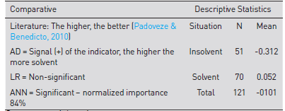
The present results were consistent with those recorded by Padoveze and Benedicto (2010, p. 264), who highlight that “in general terms, companies look forward to performing a constant growth model by gaining or amplifying markets. Thus, there is constant need of additional working capital throughout time”, because it represents the necessary resource for the company’s operational performance.
Olinquevitch and Santi Filho (2009, p. 13) also state that “The variable Net need of Working Capital is the main determinant of companies’ financial situations. Its values show the level of necessary resources to keep the business turning. Different from investments in Fixed Assets, which involve long-term decisions with slow capital recovery, calculations composing the Net Need of Working capital express short-term fast-effect operations. Changes in storage policies, in the credit policy and in purchase policy have an immediate effect on cash flow”.
According to Olinquevitch and Santi Filho (2009), the assessment of, as well as the follow-ups on, Need of Working Capital, are true signs of a company’s financial situation.
None of the solvent companies were classified as Type VI ‘high risk’ extract (Table 8); however, OGX Petróleo, which was defined as insolvent, was classified as Type I ‘Excellent’ extract. If the three best models classified OGX Petróleo as insolvent in the structure type assessment, its financial situation would go unnoticed.
4.5.3 Assessing the financial structure type
Financial Structure Types were proposed by Fleuriet et al. (1978) and expanded by Braga (1991), who added two more levels to them (Table 8). The indicator used in the current study represents a proxy recording value 1 for Type I, which increased to 6 for Type VI Financial Structure, i.e., companies classified as 1 were in the ‘Excellent’ extract, whereas companies classified as 6 were in the ‘high risk’ extract.
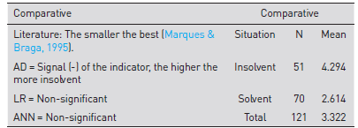
The indicator ‘Financial Structure Type’ was representa- tive in the stepwise method and in the trial and error process, which generated the discriminant analysis indices. This analysis demonstrated that the coefficient of the indicator was consistent with information in the literature. The present results showed the same behavior (Table 9).
Table 9 Summary of results recorded for indicator X8 - Financial Structure Type.
Source: own elaboration.
The Wilks’ Lambda Test applied to the discriminant analysis model was the most significant one. It recorded the lowest value (0.562), and this outcome shows the high power of this indicator in distinguishing groups. Despite the relevance of this indicator to the discriminant analysis, it was not significant in the other final models. The fact that the indicator was measured as a proxy from 1 to 6 may have influenced its exclusion when it was used with other financial indicators.
4.5.4 Reflections on liquidity thermometer and balance in treasury
According to Minussi et al. (2002) and Vieira (2008), the more negative the value recorded for Balance in Treasury, the greater the use of short-term resources from financial institutions; thus, companies’ financial situation will tend to be worse. Horta (2010) stated that the Liquidity Thermometer method assures a financial reserve to be used in occasional NWC expansion, mainly in expansions of a seasonal nature. The temporary need of working investments can be supported by the existing balance limit, as long as they are not covered by long-term financing (Padoveze & Benedicto, 2010).
Both treasury balance and the liquidity thermometer recorded negative values for insolvent companies and positive values for the solvent ones (Table 10). However, the liquidity thermometer composed two of the presented final models; the positive value recorded for solvent companies was corroborated by the positive signal of the liquidity thermometer in the discriminant analysis, which indicated that the higher the value, the greater the probability of company solvency.
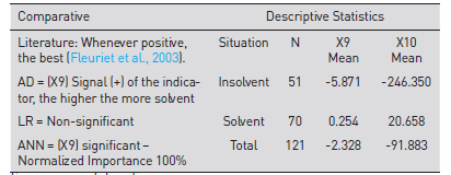
The liquidity thermometer presented normalized significance of 100%, and it explained the variation faced by the forecasted value of the neural network (output). This outcome represented the most important indicator for the best model found because it corroborated the statement by Padoveze and Benedicto (2010, p. 262), according to whom treasury bills “should be used to calculate corporate liquidity and solvency capacity in the short term”.
Results recorded for the liquidity thermometer were consistent with those recorded by Horta (2010), when the liquidity thermometer was used to assess many sectors, namely: the basic material (solvent = 0.011 and insolvent = -0.003), cyclical consumer goods (solvent = 0.010 and insolvent = -0.032) and non-cyclical consumption goods sectors (solvent = 0.002 and insolvent = -0.047); as well as the economic sectors of industrial goods (solvent = -0.133 and insolvent = -0.133), construction and transport (solvent = 0.004 and insolvent = -0.219) and of IT and telecommunications (solvent = -0.007 and insolvent = -0.385). He used the Balance in Treasury on Asset; however, this method did not appear to be significant in his models.
Empirical results based on the means recorded for Balance in Treasury were consistent with the study by Minussi et al. (2002), who used the Balance in Treasury on Net Revenues in their research and recorded a value of -0.01 for solvent companies and 2.90 for insolvent ones. According to the aforementioned study, “sampling data clearly reflects the difficulty faced by insolvent companies in operationally financing themselves, so they tend to intensively use erratic sources” (Minussi et al., 2002, p. 121).
4.5.5 Analysis of net equity on total liabilities
The indicator Net Equity on Total Liability was proposed by Altman, Baydia and Dias (1979) as an attempt to adapt indicators found in the original model by Altman (1968) to the Brazilian context. Altman, Baydia and Dias (1979, p. 22), paid close attention to the characteristics of their sample. They found that “many companies do not have papers in the stock market, so it is impossible to measure the equity of the market value (number of papers issued multiplied by the last quotation in the stock market)”. Thus, they used the Net Equity on Total Liability to generate a new indicator.
The indicator Net Equity on Total Liability’ is a Debt/ Structure indicator, i.e., a financial-leverage indicator. Soares and Rebouças (2015, p. 56) state that "this indicator associates ‘Net Equity’ with ‘Third Capital’, and this association can be understood as a risk measure reversed through the leverage the company is subjected to”.
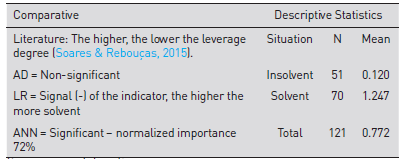
The assessed sample presented lower values for insolvent companies, whereas solvent companies recorded higher values (Table 11). Such a trend is also corroborated by the signal generated through the logistic regression, wherein companies showing high values for these indicators were possibly classified as solvent. The Net Equity on Total Liability was also useful in explaining the 72% variation in the forecasted value (output) of the neural network of normalized significance.
Table 11 Summary of results recorded for indicator X16 - Net Equity on Total Liability.
Source: own elaboration.
Results were consistent with empirical studies by Altman, Baydia and Dias (1979), who recorded a mean value of 0.35 and 1.14 for insolvent and solvent companies respectively (Table 11). These results also match a study by Soares and Rebouças (2015), who assessed public companies in Brazil and recorded a mean value of -0.185 for insolvent companies and 1.040 for the insolvent ones. According to Soares and Rebouças (2015), this indicator was important for all techniques developed in their study.
It may be assumed that the higher the value presented by the indicator, the lower the leverage performed by the company, since indicators were used to measure the proportion of resources owned by companies in relation to third resources in the capital structure. On the other hand, the lower the value recorded for this indicator, the higher the company’s leverage. The present results demonstrate that, based on the approached empirical studies, companies tend to be more leveraged.
4.5.6 Considerations about asset turnover
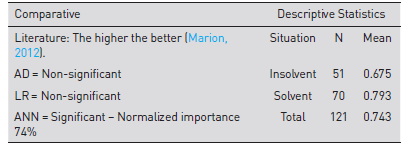
Asset Turnover is a profitability indicator that, according to Marion (2012, p. 158), means “companies efficiency in using their Assets in order to generate real sales. The more efficiently assets are used, the more sales are generated”. Padoveze and Benedicto (2010) consider that it is worth having the greatest turnover possible, because the profit/margin in the goods or services offered by the company (revenue) lead to the possibility of generating higher profit and better profitability. They also state that “if the main profitability element is revenue, the investment turnover (of the asset) is the way” (Padoveze & Benedicto, 2010, p. 122).
The Asset Turnover indicator reached 74% normalized significance to explain the variation in the neural networks (Table 12); it recorded a higher mean turnover for solvent companies.
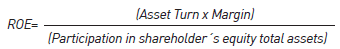
Results of neural networks which were beyond the indicator X17 - Asset Turnover. Indicators X25 - Net Margin - and X31 - Net Equity on Assets - were significant. According to Padoveze and Benedicto (2010, p. 131), these indicators composed the DuPont Model, which was “adapted to the profitability analysis of the net asset, according to the shareholder’s perspective”. According to them, the DuPont Model formula is presented in Equation 3, wherein ROE means Return on Equity.
 (3)
(3)
Padoveze and Benedicto (2010, p. 131) make it clear that the adapted DuPont Model “introduces an additional attention element. The lower the company’s own capital participation (NE), the higher its profitability, according to the composition of the formula”. Therefore, the model recommends the intense use of third capital. According to these authors, it is a financial leverage model focused on traditional finance theory, which concerns an optimal capital structure, allowing companies to improve their value through leverage.
The indicator ‘Return on Net Equity” (ROE) was not found in previous studies, which were the source of indicators selected for the present research. The Analysis of the adapted DuPont Model was not the focus of the current study, but the fact that these three variables have an intrinsic relation to each other was taken into account, as shown by Padoveze and Benedicto (2010).
4.5.7. Reflections on shareholders’ net equity return
According to Padoveze and Benedicto (2010, p. 115), profitability analysis is “the most important part of financial analysis’, because it aims to demonstrate the return of the invested capital and elucidate the determinants of such profitability. The aforementioned authors emphasize that shareholders’ Net Equity Return is the main indicator within profitability analysis, since it assesses the owners’ capital from the shareholders’ perspective. This method uses the equity of the balance sheet to analyze profitability.
Results recorded for Shareholders’ Net Equity Return are shown in Table 13; the mean values recorded for the sample were consistent with the literature. This outcome was reinforced by results recorded for the discriminant analysis, which showed positive signals and indicated that the higher the value recorded for the Shareholders’ Net Equity Return, the greater the probability of the company being solvent. The indicator reached 84% normalized significance level, and explained the variation in the forecasted value (output) of the neural network.
Table 13 Summarized results recorded for the indicator X20 - NE profita-bility.
Source: own elaboration.
Matarazzo (2010, p. 115) highlights that the function of the Shareholders’ Net Equity Return shows the profitability rate of the owned capital, “as net profit is excluded from inflation, Shareholders’ Net Equity Return rate is real”, thus, it can be compared with other market returns.
The present results converge to those in studies by Kanitz (1978), who states that the Shareholders’ Net Equity Return is, on average, three times higher for solvent companies than for the insolvent ones. According to Kanitz (1978, p. 82), “one of the characteristics of a broken company is the drastic drop in profitability”. The present study also coincided with a study by Brito (2005), who recorded the mean value for insolvent companies as -0.36 and 0.17 for solvent ones.
4.5.8. Assessment of the net margin
According to Marion (2012, p. 158), the Net Margin “means how many cents of real sales remain after all expenses are deducted (including income tax)”; it is evident that the higher the margin, the better. Based on Matarazzo (2010), the Net Margin shows how much the company earns on profit over sales.
The mean values recorded for the sample were consistent with the literature, i.e., the higher the value presented by the indicator, the better the profit margin reached by the company in relation to the volume of net sales in the period (Table 14). Such an amount is confirmed by the signals presented either by discriminant analysis or logistic regression. Based on this outcome, the higher the net margin value, the greater the probability of the company being solvent. The indicator also presented 78% normalized importance for the neural network model.
Table 14 Summarized results recorded for indicator X25 - Net Margin.
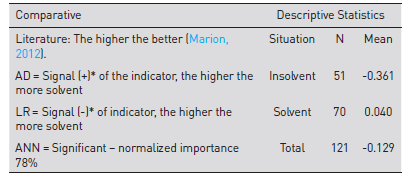
*Signals presented by the discriminant analysis and by the logistic regression were opposite, due to the way the calculation was done; however, when signals were reversed, they presented the same trend in these indicators; which, in the present case (AD = ‘+’ and LR = ‘-’) is: the higher, the better.
Source: own elaboration.
The indicator Net margin of the Traditional Financial Analysis Model stood out among the other indicators, because it was found in four of the proposed indicator groupings. Besides, it is integrated within the three models (AD, LR and ANN) presenting the highest significance in the analysis. The present results were consistent with the empirical study developed by Brito (2005), who recorded a mean value of -0.11 for insolvent companies and 0.01 for the solvent ones when assessing public companies in Brazil.
4.5.9. Analysis of debt breakdown
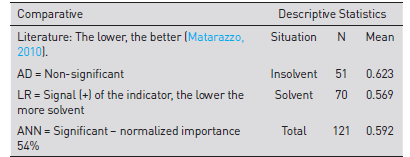
Debt breakdown is a Debt/Structure indicator which, according to Matarazzo (2010, p. 90), shows “the short-term obligation percentage in relation to total obligations”. As these authors state, the lower the result, the better the company.
According to Marion (2012), companies operating with shorter-term debts are in an unfavorable position, and it impairs their financial situation. Matarazzo (2010) also argues that one thing is having shorter-term debts that need to be paid within shorter-term incomes, and another thing is to have longer-term debts that have time enough to be paid.
The indicator Debt Breakdown shown in Table 15 appeared to be significant in the present research, because the mean value recorded for solvent companies was lower than the one recorded for the insolvent ones. This finding was reinforced by the signal of the logistic regression model, which was consistent with the literature, i.e., the higher the signal, the greater the probability of the company being solvent. The indicator was also significant for the neural networks model.
Table 15 Summarized results recorded for the indicator X28 - Debt Breakdown.X
Source: own elaboration.
The present results were consistent with those recorded by Castro Junior (2003, p. 112), who recorded a mean value of 0.5428 for insolvent companies and 0.4085 for solvent ones. Castro Junior (2003) also states that what really matters is to prove the initial hypothesis; the longer the short-term debt, the greater the probability of the company being classified as insolvent. This hypothesis was corroborated by Castro Junior (2003) in 5 of the 7 generated final models.
4.5.10 Assessing the net equity on assets
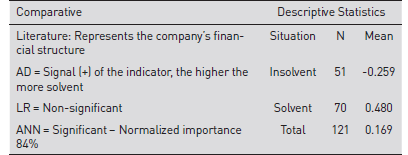
Padoveze and Benedicto (2010, p. 115) observe that the indicator Net Equity on Assets is used to measure asset financing because it aims to measure companies’ financing structure. According to them, this indicator shows the fraction of the asset financed by the owned capital; thus, it demonstrates the reflex of financial leverage policies.
The Net Equity on Assets indicator recorded a negative value for insolvent companies and positive values for solvent ones (Table 16). Such a relation was also reinforced by the discriminant analysis model, which recorded a positive signal for the coefficient. Based on this outcome, the higher the Net Equity on Assets, the greater the probability of the company belonging to the group of solvent companies, i.e., leveraged companies present a greater probability of being insolvent.
Table 16 Summarized results recorded for indicator X31 - Net Equity on Assets.
Source: own elaboration.
Based on the analysis applied to indicator X17 - Asset Turnover -, which took into consideration the adapted DuPont Model, and according to Padoveze and Benedicto (2010), this indicator becomes a financial leverage model focused on traditional financial theory. According to Durand (1952), if the company grows beyond the optimal capital structure, even when it reaches better results, it will face unjustified bankruptcy costs.
The present results are consistent with those recorded by Brito (2005) who, by studying public companies, recorded lower values for insolvent companies (mean 0.34) and higher values for solvent ones (mean 0.56).
5. Conclusion
The best model for each technique was presented by comparing the techniques used to forecast companies’ insolvency. The superiority of artificial neural networks over logistic regression, as well as of logistic regression over discriminant analysis, was noteworthy. These results were confirmed by the success levels presented by the techniques: discriminant analysis, 90.9%; logistic regression, 90.9%; and artificial neural networks, 97.8%.
Indicators belonging to the Fleuriet Model were significant for the groupings. The contributions from the Fleuriet Model became clearer when the individual participation of each indicator was assessed in the final credit granting models.
Liquidity Thermometer and the Need of Working capital were the two most representative indicators belonging to the Fleuriet Model. They contributed to the best neural network models, since they recorded 100% and 95% normalized significance respectively, and explained the variation in the forecasted values recorded for the network (output).
Results of Liquidity Thermometer showed the importance of financial calculations (treasury bills) at the time of calculating companies’ liquidity and solvency capacity in the short term.
The NWC was the only indicator belonging to all proposed groupings, it became the main determinant of companies’ financial situations. Overall, companies look forward to performing a constant growth model by expanding or gaining markets; thus, there is always the need of additional working capital throughout time, because their value represents the necessary resource level to maintain business turnover and operational performance. Working Capital, Financial Structure Type and Balance in Treasury stood out among the Flueriet Model indicators.
The Net Margin stood out among calculations of the Traditional Financial Analysis Model. Shareholders’ Net Equity Return was another important indicator, so it was selected for the discriminant analysis model and for the artificial neural networks. Net Equity on Assets was another indicator participating in the discriminant analysis and artificial neural networks techniques, since it was consistent with traditional financial theory.
One of the limitations of the present study lies in the impossibility of generating models per specific sector, something that could have improved either the precision of the models or to broaden understanding of factors determining the insolvency of public companies in Brazil. Further studies are recommended, because they will make it possible to develop hybrid models based on Computer Intelligence to improve credit risk modeling accuracy and to assess the contribution from the adapted DuPont Model recommended by Padoveze and Benedicto (2010) for credit risk analysis. The indicators used to calculate Return on Net Equity (ROE) were significant for the artificial neural networks model.
The present study can elucidate some of the characteristics of insolvent companies in the sample. These contributions are essential for credit risk studies and to help develop the topic through the comparison of analysis techniques (DA, LR and ANN). The general application of these methods can be seen in the forecasting capacity of the generated model in the balance sheet analysis applied to insolvent companies, one year before they issued a preventive bankruptcy filing or judicial recovery request.
Finally, indicators effectively contributed to forecasting companies’ insolvency. Enhancements in the methodologies used, as well as the evolution of forecasting techniques, helped the personnel in charge to maintain business liquidity and to avoid bad debt or even bankruptcy.

