Artículo de Investigación/Research Article

Dynamic Inverse Problem Solution Using a Kalman Filter Smoother for Neuronal Activity Estimation

Eduardo Giraldo-Suárez¹, Jorge I. Padilla-Buriticá², César G. Castellanos-Domínguez³

¹Programa de Ingeniería Eléctrica, Universidad Tecnológica de Pereira, Pereira-Colombia, egiraldos@utp.edu.co

²Programa de Ingeniería Electrónica, Universidad Nacional de Colombia sede Manizales, Manizales-Colombia, jipadilla@unal.edu.co

³Programa de Ingeniería Electrónica, Universidad Nacional de Colombia sede Manizales, Manizales-Colombia, cgcastellanosd@unal.edu.co

Fecha de recepción: 25 de enero de 2011 / Fecha de aceptación: 16 de septiembre de 2011

Abstract

This article presents an estimation method of neuronal activity into the brain using a Kalman smoother approach that takes into account in the solution of the inverse problem the dynamic variability of the time series. This method is applied over a realistic head model calculated with the boundary element method. A comparative analysis for the dynamic estimation methods is made up from simulated EEG signals for several noise conditions. The solution of the inverse problem is achieved by using high performance computing techniques and an evaluation of the computational cost is performed for each method. As a result, the Kalman smoother approach presents better performance in the estimation task than the regularized static solution, and the direct Kalman filter.

Keywords: Inverse problem, neuronal activity, Kalman filter, physiological model.

Resumen

En este artículo se presenta un método de estimación de la actividad neuronal sobre el cerebro usando un filtro de Kalman con suavizado, que tiene en cuenta en la solución del problema inverso, la variabilidad dinámica de la serie de tiempo. Este método es aplicado sobre un modelo realista de la cabeza, calculado con elementos finitos de frontera. Se presenta un análisis comparativo entre diferentes métodos de estimación y el método propuesto sobre señales EEG simuladas para diferentes condiciones de relación señal a ruido. La solución del problema inverso se hace utilizando computación de alto desempeño y se presenta una evaluación del costo computacional para cada método. Como resultado, el filtro de Kalman con suavizado presenta un mejor desempeño en la tarea de estimación comparado con la solución estática regularizada, y la solución dinámica sin suavizado.

Palabras clave: Problema inverso, actividad neuronal, filtro de Kalman, modelo fisiológico.

1. Introduction

The identification of dynamic behavior in neuronal activity is a main part of the brain pathologies treatment. Commonly, the estimation of neuronal activity is made up from electroencephalography (EEG) signals measured noninvasively from the head (scalp recordings). The EEG signals allow a better temporal resolution in contrast with other techniques like the functional Magnetic Resonance Imaging which brings better spatial resolution. EEG source reconstruction or neuronal activity estimation is known to be an ill posed inverse problem as there are an infinite number of different solutions that give rise to identical scalp recordings. Until recently, most attempts to solve the inverse problem were based on EEG signals at one single time point. However, since neuronal activity has an inherent strong spatial and temporal dynamics, the solution of the inverse problem must take into account these dynamics as additional constraints (Peralta et al., 1998; Pascual et al., 1999; Baillet et al., 2001). This can be done, by choosing appropriate dynamic models that pose dynamics constraints in the solution (Yamashita et al., 2004; Grech et al., 2008; Giraldo et al., 2010).

For example, in Galka et al. (2004) autoregressive (AR) models are used for modeling neuronal activity, assuming that the dynamical model is linear and depends of the previous states of neuronal activity. As a result, the inclusion of dynamical constraints improves the performance of the instantaneous case. On the other hand, there are different problems that must be considered in the implementation and development of the dynamic inverse solution. First of all, dynamic estimation of neuronal activity is a high dimensional problem and its implementation has a high computational load. However, the main restriction is the selection of the dynamical model.

A physiological based model allows a better description of the system dynamics. In Robinson et al. (2007) is discussed a differential equation that can describe satisfactorily the dynamic behavior of neuronal activity including the physiological features of EEG signals. For example, in Barton et al. (2009) a simple dynamic model with resonant behavior is used according to the physiological features of EEG signals. Neuronal activity is estimated through Kalman Filtering (KF) and the high dimensionality problem is addressed by using a modified KF that reduces the problem to a set of low dimensional KFs, one at each considered source. Anyway, when dynamic model performance is evaluated over real EEG signals they obtain problems in spatial coupling as a result of the implementation proposed in Barton et al. (2009) and because the spatial term of the dynamic model is inaccurate. It is possible to improve the performance of the decoupling method proposed in Barton et al. (2009) using methods of filter partition as proposed in Sitz et al. (2003) or high performance computing (Long et al., 2006). Additionally, the estimated solution can be improved through methods of smoothing that consider the variability of all the data (Kaipio et al., 1999; Tarvainen et al., 2004). However, smoothed solutions involve high computational load, and high capacity for storage information in intermediate steps.

In the other hand, the solution of the inverse problem do not depends only of the dynamic model selection but also of the adequate lead field matrix that relates the sources associated with the signals measured on the scalp and reporting directly to the head model (Plummer et al., 2008). As head model there can be used from simple models (spherical) to complex models (finite element method, boundary element method, finite volumes, finite differences, etc.), which includes the conductivity corresponding tissues. These models allow increasing the spatial resolution of the estimated neuronal activity into the brain. However, the more we increase the resolution, the higher dimensionality we get for dynamic model of neuronal activity and the higher computational load we have, but the better mapping of neuronal activity we achieve (Deneux et al., 2006; Hallez et al., 2007). Nevertheless, selection of head model modifies the accuracy of spatial estimation but not its dynamics. For that reason, considering any head model, it is possible evaluating the performance of different methodologies of estimation for neural activity (Grech et al., 2008; Plummer et al., 2008).

This article presents an EEG source reconstruction method that solves the inverse problem in a Kalman filtering framework using a smoother approach. The methodology is applied over a realistic head model calculated with the boundary elements method (BEM). The analysis is made up from simulated EEG signals for several levels of noise. The solution of the inverse problem is achieved using high performance computing techniques. This article is organized as follows: section 2 presents methods for solving the inverse problem for the static case using a regularized solution and for the dynamic case using direct Kalman filter estimation and Kalman smoother approach, and also presents a head model using the BEM; section 3 presents the comparative analysis between the static and dynamic methods for several noise conditions. Finally, section 4 presents conclusions and future work.

2. Materials and methods

2.1 Inverse problem framework

The relationship between EEG measurements on the scalp and the current density resultant from the neuronal activity into the brain is described by the observation (1).

In (1), y denotes a vector of dimension d x 1  that contains the measures of the EEG on the scalp for d electrodes. X = (X₁^T ... X_N^T)^T denotes a 3N x 1 vector that contains the current density vectors X_i = (X_ix X_iy X_iz)^T with i = 1,2,...,N where N is the number of sources inside the brain. Matrix M has a d x 3N dimension and it relates the current density inside the brain x with EEG measurements y. M is called lead field matrix and can be calculated using Maxwell equations for a specific head model (Yamashita et al., 2004). The vector ε with d x 1 dimension is an additive random variable that represents the non-modeled features of the system, i.e. observation noise, and it can be assumed as a Gaussian distribution of the form ε ∼ G(0,σ²Σ_ε) with known covariance structure Σ_ε. The forward problem is defined as calculation of measurements y  for a given current density vector x. Therefore, (1) is used for simulation of EEG signals where any variation of ε can simulate several noise conditions.

The inverse problem is defined as the estimation of current density from a given measurements y and establish an ill posed problem since the number of scalp electrodes (dimension of y) is much smaller than the number of sources where current density of neuronal activity should be estimated (dimension of ). The inverse problem proposed in (1) is recognized as static or instantaneous since there are only used measurements in a single instant of time for estimation of . Generally, the estimation of can be obtained by minimizing the objective function given in (2).

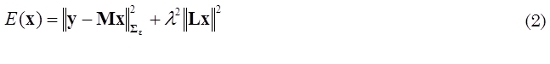
Where L is a matrix with 3N x 3N  dimension and is defined as the spatial smoothness constraint, where the ith row vector of L  acts as a discrete differentiating operator (Laplacian operator), by forming differences between the nearest neighbors of the jth source and ith source itself (Yamashita et al., 2004). The parameter λ, called regularization parameter, expresses the balance between fitting the model and the prior constraint of minimizing ǁLxǁ. The solution of this minimization problem for a given λ is obtained by (3).

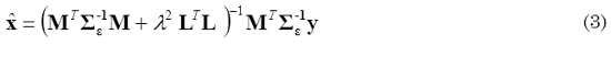
The parameter λ is calculated using methods of parameter selection as L-curve (Hansen et al., 1998). However, the obtained solution is achieved for each time independently, and it doesn’t take into account the dynamic behavior. Consequently, it is possible to consider a modification of (2) to achieve an objective function containing the spatial and temporal smoothness constraints, as shown in (4).

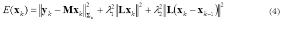
where y_k is the EEG measurements at time instant k, X_k  is the state vector that correspond to the neuronal activity in each source into the brain at time k, and λ₁, λ₂ are defined as regularization parameters. Additionally, the interactions between neighboring sources in time can also be taken into account by including the Laplacian matrix L into the third term of (4). By introducing a new parameter A that represents a balance between the second and third terms of (4), we can combine the two penalty terms and obtain a more compact expression:

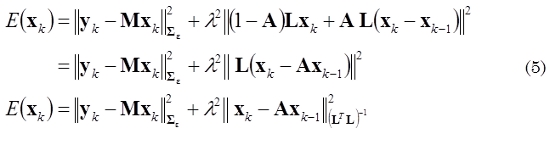
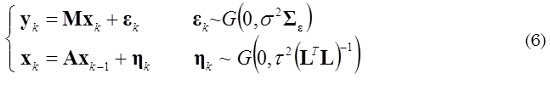
The objective function in (4) and (5) are not equivalent mathematically; however, (5) can be regarded as a different way of imposing these two kinds of constraints (spatial and temporal). Moreover, (5) can be related with a state space representation, as shown in (6).

An initial estimate (for k = 1) of the state x₁ can be obtained by any approach for solving the instantaneous inverse problem. For k = 2,…, N,  we can obtain an estimate of by minimizing (5), as given by (7).

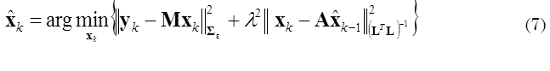
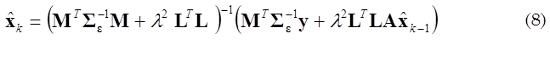
where is the estimate obtained in the previous step. The solution of (7) is given by (8).

The structure of A is selected according to a physiological based model proposed by (Robinson et al., 2007, Barton et al., 2009). In the case of a first order linear model x_k = Ax_k-1 + η_k, A is defined as follows

where a₁ considers the variability among sources in time and b₁ in space.

2.2 Dynamic estimation

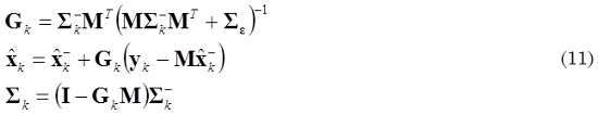
Direct computation of (8) is numerically impracticable because it requires the inverse of  M; however, the dynamic inverse problem in the case of neuronal activity estimation x_k presented in (6) is a state space formulation that could be solved through a forward Kalman filtering using the recursion given by (10) and (11), which are known as time update equation and measurement update equation, respectively.

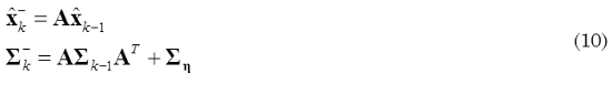
where is defined as a priori estimation of , Σ_k^- is defined as a priori covariance, and Σ_η = (L^TL)^-1 is the covariance related with η.

Therefore, the estimated neuronal activity is mapped over a realistic head model. However, in spite of is estimated for each k using only the data up through time k, it is possible to improve the precision of the estimated states using a smoother that computes a smoothed version of the estimated neuronal activity using all the available data (k = 1,2,...,N) in the experiment from the obtained results of recursion (11) in a backward recursion. This smoother applied over the Kalman filter estimation is known as the Rauch–Tung–Striebel smoother (Haykin et al., 2001) and is given by (12) for k = N - 1,...,1.

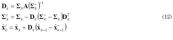
where D_k is the gain matrix of the smoother and the initial values for the backward recursion are Σ_s^N = Σ_N and .

2.3 Realistic head modeling through BEM

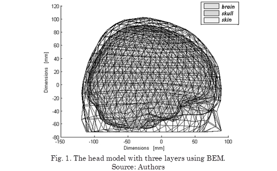
In head modeling there can be used from simple models such as spherical, to complex models like finite elements, BEM, finite volumes, finite differences, etc. Modeling with the BEM presents a middle point of complexity between the named models, obtaining a more realistic approximation of the head model while it keeps some properties of simple spherical models (i.e. uniform conductivity). The head models vary their complexity with the number of layers (one layer: the brain; two layers: brain and skull; three layers: brain, skull and skin; four layers: brain, skull, cerebrospinal fluid, skull and skin) as described in (Plummer et al., 2008).

The BEM model consists of a set of point located over every layer of head model and that form the vertices of a set of triangles. In this way, the realistic model obtained corresponds to an approximation through the set of triangles for every layer which are considered isotropic conductivities in the same way as is done for the spherical model. In Table 1 are described the properties of the realistic head model computed by BEM.

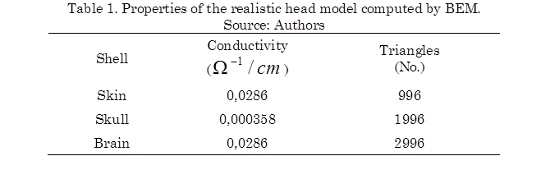
Thus, the lead field matrix M involves spatial relationships between sources located within the brain (inner layer) with located electrodes over the skin (outermost layer). Fig. 1 shows the head model with three layers using BEM.

3. Results and discussion

3.1 Experimental setup

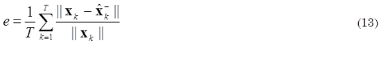
Three cases are analyzed in this article for estimation of neuronal activity: for the static case the estimation is achieved using the regularized Tikhonov solution proposed in (3). For dynamic cases, the estimation is performed using two solutions: the direct Kalman filter approach proposed in (10) and (11) and the Rauch–Tung–Striebel smoother approach presented in (12). For the dynamic cases, brain dynamic is approximated through a first order linear model with the structure of A proposed in (9). A comparative analysis is performed considering individuals contributions in the structure of A for the variability among sources in time and space. In this way, an estimation error e given by (13), according to (Grech et al., 2008) is used for each trial:

In this line, and in order to consider the relative contribution to the filter performance of the several parts of the process model for the dynamic inverse problem, the following cases are to be considered: 1) static case solution described in (3); 2) first order model given in (6) without spatial coupling (b₁ = 0) using direct Kalman filter approach; 3) first order model given in (6) with spatial coupling using direct Kalman filter approach; 4) first order model given in (6) without spatial coupling (b₁ = 0) using the Rauch–Tung–Striebel smoother approach; and 5) first order model given in (6) with spatial coupling using the Rauch–Tung–Striebel smoother approach.

A major issue regarding to the inverse solution task is obtaining meaningful evaluations of the estimation results and its performance, because locations of true sources are not available for comparison when working with real EEG data. Instead, the most common approach is to use simulated EEG data where underlying sources are known. Two types of sources will be considered: sources randomly located near the surface of the brain and sources randomly located deep in the brain. Nonetheless, to generate a simulated EEG dataset for this purpose requires selecting a model for the brain dynamics, which displays complex spatio-temporal behavior. Here, the temporal dynamics are suggested to be modeled using a linear combination of sine functions whose components are evenly spaced in the alpha band (8 – 12 Hz), which is selected since the clinical data used in typical real EEG recordings display prominent alpha activity (Barton et al., 2009). Specifically, the simulated brain dynamics where generated for 256 time points, assuming a sampling rate of 256 Hz.

The performance of the inverse solutions is compared with simulated EEG data for the following values of signal noise ratio (SNR): 5 dB, 10 dB, 15 dB, 20 dB and 25 dB for each type of source. Besides, 25 repetitions of one second of synthetic EEG data, according to 10-20 system, are generated from the simulated current densities by multiplication with the lead field matrix  M. Prior to computing an inverse solution, we define a discretized solution space consisting of 7x7x7 mm gray matter grid points (sources), as recommended in (Barton et al., 2009). These sources cover the cortex and basal ganglia. At each source, the 3D local current vector is mapped, as usual, to the 19 electrode sites for the 10-20 system. Finally, an evaluation of the computational load is performed for static case using regularization and first order dynamic case using direct Kalman filtering and the Rauch–Tung–Striebel smoother approach.

3.2 Estimation results

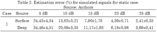
The obtained results for the static case solution of (1), when considering several SNR, are shown in Table 2, where a regularized solution is used to solve the inverse problem of (3). In this case, a Tikhonov solution with L-curve method for parameter selection is used (Hansen et al., 1998). It can be seen that the obtained results are similar to the outcomes given in (Grech et al., 2008), namely, the performance of the considered algorithm is highly dependent of the noise.

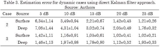
On the other hand, when temporal constraints are included in the solution of the inverse problem, the solution of the inverse problem could be improved. In the case of a first order dynamic model, where the neuronal activity is estimated using Kalman filter, the obtained results are shown in Table 3, which are similar with those outcomes given in (Barton et al., 2009), for time invariant parameters (calculated offline). For example, when looking to the first order model without spatial coupling (case 2), the results are not as good as in the case of the first order model with spatial coupling (case 3). It must be quoted that similar result, for the considered variations of the dynamic model, where obtained in (Barton et al., 2009).

Nonetheless, it is clear that estimated solution takes into account only the information available up to k. It is possible to improve the precision of the estimated solution using a smoother that computes a smoothed version of the estimated neuronal activity using all the available data (k = 1,...,N) in the experiment from the obtained results of direct Kalman filter approach. Therefore, applying the Rauch–Tung–Striebel smoother approach over the cases 2 and 3, the obtained results are shown in Table 4.

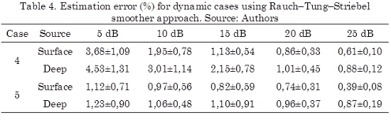
Hence, a comparison between Tables 3 and 4 show that the smoothed solution improves the precision of the estimation and reduces the dispersion of the data. However, this improvement leads in high computational load because it is necessary to save the estimated and covariance Σ_k^- and Σ_k for all k.

3.3 Computational load

In order to evaluate the performance of the solutions from a computational load point of view using the high performance computing techniques, an evaluation of the estimation process time is performed for static case, dynamic case using a direct Kalman filter approach and a Rauch–Tung–Striebel smoother approach. This analysis is performed over a single computer with dual core of 2.6 GHz processor, 2 GB of RAM DDR3 and 120 Gb of hard disk. In order to address the limitation of large scale computations, we arrange the Kalman filtering computations such that the data intensive aspects of the algorithm can run in parallel. The results of this evaluation for 25 repetitions of each case are shown in Table 5.

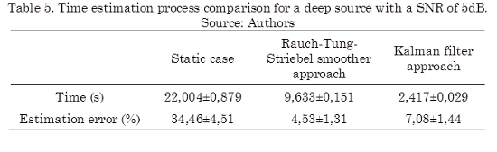
It is noticeable from Table 5, that the estimation time for the dynamic cases using direct Kalman filter approach is 10 times less than the static case. In particular, the estimation time of using the Rauch-Tung-Striebel smoother approach is 5 times more than the direct Kalman filter because it requires an additional smoothness step but principally because it is necessary to save a lot of information for this step. Even so, the smoother approach requires almost the half of time than the static case. Besides, it can be seen clearly that a lower estimation error is achieved by the Rauch-Tung-Striebel smoother approach since the estimated model takes into account the variability of the whole signal. Therefore, the Rauch–Tung–Striebel algorithm must be considered in applications where an elevated precision is highly desirable over the computational cost.

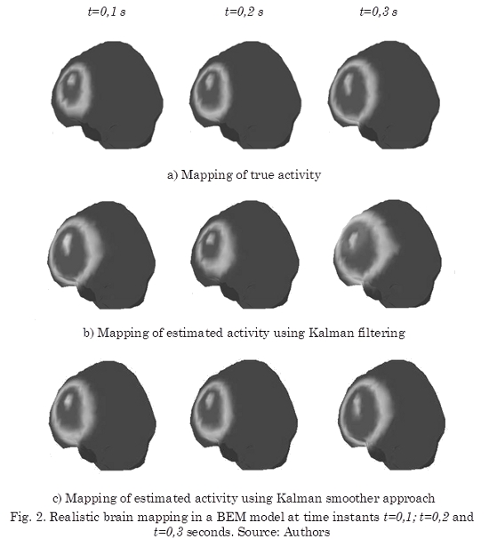
Finally, the estimated solutions are mapped over a realistic head model calculated with BEM as shown in Fig. 2, where the pallid sectors into the brain correspond to the estimated activity. It is clear by comparison with the true activity (Fig. 2a) that the dispersion introduced by the covariance in the Kalman filtering (Fig. 2b) is reduced by the Kalman smoother approach along time (Fig. 2c). The mapped activity offers an interesting tool for diagnostic support because it shows the activity into the brain related with the EEG events when is use for real EEG signals.

4. Conclusions and future work

In this paper, we have addressed the dynamical inverse problem of EEG signals for estimation of neuronal activity, using a Kalman filtering smoother approach. According to the obtained results, this approach improves the precision of the estimation over the Kalman filter but increases the computational load. Despite that, both the Kalman filter and Kalman filter approach are faster than the static case, and more precise.

As expected, the more elaborate a dynamic model is applied, the more the resulting inverse solutions will be able to explain the observed EEG data. These results were confirmed for each case study in this paper for simulated signals over several SNR values where the first order model that include in the structure of A the variability among sources in time and space presents reached the better performance in comparison with the static case. In order to improve the estimated solutions, more complex models could be used. However, for the Kalman smoother approach, these elaborated models could increase the computational load, and the reduction of the estimation error could not be relevant.

For future work, a Kalman smoother approach applied over a dynamic model with time varying parameters is proposed; with the intention of achieve a better performance of the estimator.

5. Acknowledgments

Authors would like to thank “COLCIENCIAS”, “Universidad Tecnológica de Pereira”, and “Universidad Nacional de Colombia, sede Manizales” for the financial support on the project “Sistema de Identificación de Fuentes Localizadas Epileptogénicas Empleando Modelos Espacio Temporales de Representación Inversa”.

Referencias

Baillet, S.; Mosher, J.; Leahy, R. (2001); Electromagnetic Brain Mapping, IEEE Signal Processing Magazine, 18(6), 14-30.         [ Links ]

Barton, M.; Robinson, P., Kumar, S., Galka, A., Durrant-White, H., Guivant, J. and Ozaki, T. (2009); Evaluating the Performance of Kalman-Filter-Based EEG Source Localization, IEEE Transactions on Biomedical Engineering, 56(1), 122-136.         [ Links ]

Deneux, T. and Faugeras, O.; (2006); EEG-fMRI fusion of non-triggered data using Kalman filtering, 3rd IEEE International Symposium on Biomedical Imaging: Nano to Macro, 1068-1071.         [ Links ]

Galka, A., Yamashita, O., Ozaki, T., Bizcay, R. and Valdez-Sosa, P. (2004); A solution to the dynamical inverse problem of EEG generation using spatiotemporal Kalman Filtering., Neuroimage, 23(1), 435-453.         [ Links ]

Giraldo, E.; den Dekker, A.J.; Castellanos-Dominguez, G. (2010); Estimation of dynamic neural activity using a Kalman filter approach based on physiological models, Proceedings of the 32nd Annual International Conference of the IEEE Engineering in Medicine and Biology Society, 2914-2917.         [ Links ]

Grech, R., Tracey, C, Muscat, J., Camilleri, K.; Fabri, S.; Zervakis, M.; Xanthoupoulos, P., Sakkalis, V. and Vanrumste, B., (2008);. Review on solving the inverse problem in EEG source analysis, Journal of NeuroEngineering and Rehabilitation, 5(25).         [ Links ]

Hallez, H., Vanrumste, B., Grech, R., Muscat, J., Clercq, W., Velgut, A., D'Asseler, Y., Camilleri, K., Fabri, S., Van Huffel, S. and Lemahieu, I. (2007); Review on solving the forward problem in EEG source analysis, Journal of NeuroEngineering and Rehabilitation, 4(46).         [ Links ]

Hansen, C. (1998); Rank-Deficient and Discrete III-Posed Problems: Numerical Aspects of Linear Inversion, Society of Industrial and Applied Mathematics.         [ Links ]

Haykin, S.; (2001); Kalman filtering and Neural Networks, John Wiley and Sons Inc.         [ Links ]

Kaipio, J.P., Juntunen, M.; (1999); Deterministic regression smoothness priors TVAR modelling, in Proc. IEEE ICASSP-99, 1693--1696.         [ Links ]

Long, C., Purdon, P., Temereanca, S., Desai, N., Hamalainen, M. and Brown, E, (2006); Large scale Kalman Filtering Solutions to the Electrophysiological Source Localization Problem, A MEG Case Study., Proceedings of the 28th IEEE EMBS Annual International Conference, 4532-4535.         [ Links ]

Pascual-Marqui, R. (1999); Review of Methods for Solving the EEG Inverse Problem, International Journal of Bioelectromagnetism, 1(1), 75-86.         [ Links ]

Plummer, C., Simon-Harvey, A. and Cook, M. (2008); EEG source localization in focal epilepsy: Where are we now?, Epilepsy, 49(2), 201-218.         [ Links ]

Robinson, P. and Kim, J. (2007); Compact Dynamical Model of Brain Activity, Physical Review E, 75(1), 0319071-03190710.         [ Links ]

Sitz, A. and Kurths, J. and Voss, H. U. (2003); Identification of nonlinear spatiotemporal systems via partitioned filtering, Physical Review E, 68( 1), 0162021-0162029.         [ Links ]

Tarvainen, M., Hiltunen, J., Randa-aho, P., Karajalainen, P.; (2004); Estimation of non-stationary EEG with Kalman Smoother approach: an application to event related synchronization (ERS), IEEE Transactions on Biomedical Engineering, 51(3), 516-525.         [ Links ]

Yamashita, O., Galka, A., Ozaki, T., Bizcay, R. and Valdez-Sosa, P., (2004); Recursive Penalized Least Squares Solution for Dynamical Inverse Problems of EEG Generation., Human Brain Mapping, 21(1), 221-235.         [ Links ]