


 English (pdf)
 Article in xml format
 Article references
 Send this article by e-mail
 Cited by SciELO
  Cited by Google
  Similars in
SciELO
Similars in
SciELO  Similars in Google
 Permalink
1 INTRODUCTION
The transmission network expansion planning (TNEP) problem consists in determining the lowest cost of investment for new transmission assets that must be installed in a power system to attend a forecasted demand within a given time horizon [1]. The fact that TNEP has a long-lasting impact on systems operation makes it one of the main strategic decisions in power systems. Furthermore, TNEP is a non-convex, non-linear and multi-modal optimization problem which, from a computational complexity point of view is cataloged as NP-hard [2].
Several models and solution techniques have been proposed in the specialized literature to approach the TNEP problem [3]. Heuristic [4], metaheuristic [5]-[6] and exact methods [7]-[8] have been explored to tackle the TNEP problem in its different versions. Heuristic techniques are easy to implement but rather often get trapped in local optimal solutions. Metaheuristic techniques are more refined search procedures able to find better solutions than common heuristic techniques, but at the expense of higher computational time. Finally, exact methods can guarantee the achievement of optimal solutions but require a linearization of the problem, which in most cases is a challenging task and leads to neglect certain effects such us reactive power requirements. A comprehensive review of the state of the art that considers modeling, solving methods, integration of distributed generation, environmental impacts and uncertainty issues within TNEP can be consulted in [9]. Also, a classification of several studies and models of transmission expansion planning is presented in [10].
Currently, the growing levels of penetration of renewable-based generation have posed major challenges to TNEP. In [11], the authors present a multi-objective approach for determining transmission expansion plans that considers the effect of distributed generation (DG). In [12], the authors consider different operating scenarios and wind power generation for TNEP, including the optimal location of thyristor controlled series components. Other works that integrate DG into TNEP are presented in [13] and [14].
Power system security is also an important issue when deciding which new lines to add to an existing network. The most common way to keep track of security constraints is through the N-1 criterion, which establishes that the power system must continue to operate, within allowed limits, after any single contingency takes place. Several studies have been conducted in this regard. In [15], the authors propose a multi-objective approach to solve the TNEP problem considering investment costs and the N-1 security criterion. An interior point method combined with a metaheuristic technique is used to solve the problem. In [16], the authors approach the TNEP problem considering the N-1 security criterion and introducing energy storage to provide the system with operational flexibility, deferring expansion investment and reduced costs. In [17], the line outage distribution factors are used to create a contingency identification index to detect critical lines and incorporate the eventual outage of such elements within the TNEP problem. In [8], an exact method is proposed to solve the TNEP problem introducing a subset of credible contingencies. In [18], the authors propose a Benders decomposition approach to solve the TNEP considering single contingencies. The Bender cuts are used to decompose the original problem into smaller sub-problems. In general, the contingency analysis to guarantee a robust expansion plan increases the complexity of the TNEP. This is confirmed by another work [19] in which the authors are forced to reduce the maximum number of lines in each branch to only one and do not consider the possibility of adding new lines in all corridors. When considering security criteria, TNEP is usually solved in two phases [20]. In the first one, the problem is approached neglecting the effect of contingencies; in the second, new lines are added every time a contingency makes the system operation unfeasible. The main drawback of this approach is the fact that, when dividing the optimization problem into two different sub-problems, the optimality of the solution is not guaranteed. Consequently, the problem must be modeled considering the complete set of contingencies. This approach is developed in [8] by using mixed integer linear programing (MILP) methods. Nevertheless, for medium and large size power systems the time required to solve a MILP problem increases exponentially, which sometimes makes the inclusion of security constraints intractable, thus forcing planner engineers to develop strategies in order to reduce the search space. In this paper, we have approached the TNEP problem with a metaheuristic technique. These methods are well suited for solving complex mathematical problems and have been successfully applied to approach the TNEP problem as reported in [21], [22] and [23]. Given the fact that TNEP is represented by a multi-objective optimization problem, the NSGA-II (Non-dominated Sorting Genetic Algorithm II) was implemented for its solution. This algorithm has several characteristics that make it suitable for multi-objective optimization, such as reduced computational complexity for non-dominated sorting and the use of elitism that speeds up its performance. Also, the NSGA II does not use additional parameters for preserving the diversity of the solutions. This algorithm has proven to be effective in tackling the multi-objective TNEP problem as shown in [15], [24] and [25].
Two conflicting planning objectives have been considered in the proposed TNEP model: the minimization of costs and the maximization of security. The first one considers the cost of adding new circuits and small-scale generators to the system, while the second one consists in guaranteeing a feasible operation under both normal operating conditions and single contingencies. The second objective is modeled through the weighted transmission loading relief (WTLR) indexes proposed in [26]. Note that none of the above-mentioned studies use WTLR indexes to account for contingencies. The novelty of the proposed model lies on the use of such indexes that are expressed in terms of shift and power distribution factors. Including such factors allows the model to implicitly consider security constraints. Also, the possibility of adding small-scale controllable generation units is considered. Therefore, this paper aims to contribute to the discussion of new TMEP modeling approaches. In summary, the main features and contributions of this paper are the following:
A new model for the TNEP problem, that integrates security constraints (N-1 criterion) thought WTLR indexes, is proposed.
A multi-objective algorithm was implemented to solve the proposed model, thus allowing to find trade-offs between the costs of expansion plans and their levels of security.
Furthermore, the possibility of introducing small-scale or distributed generation into the expansion plan was integrated in the model. The controllability of this type of generation technologies plays a key role in the security levels of the system; in the case of non-controllable technologies, there is no guarantee they contribute to higher security levels due to the inherent uncertainty of generation levels. In this case, only controllable DG technologies such as turbine gas, small hydo, reciprocating engines, and microturbines were considered. Under this assumption it is possible to reduce the number of transmission assets required in the transmission plan and contribute to higher security levels.
The remaining of this document is organized as follows. Section 3 presents the mathematical formulation of the TNEP considering WTLR indexes. Section 4 describes the metaheuristic method applied to solve the proposed model. In Section 5, several tests are performed using the Garver system and the IEEE 24-bus reliability test system. Finally, Section 6 presents the conclusions.
2. MATHEMATICAL FORMULATION
2.1 Objective functions
The objective functions considered in the proposed model are given by (1) and (2). The first objective function is composed of five terms. The first two terms indicate the cost of adding new transmission lines and small-scale generators, respectively. In this case, the binary variables w l and z k are used to indicate the existence of new transmission lines and generators, respectively. The third and fourth terms indicate the operating costs of existing and new generators, respectively. The last term indicates the cost of unserved demand. Equation (2) represents the minimization of the maximum absolute value of the WTLR indexes, which are defined in the next sub-section. Note that this forces WTLR indexes to move towards zero. If such indexes are zero, it means that no overload is present, neither in the base case nor under any contingency.


2.2 Constraints regarding WTLR indexes computation
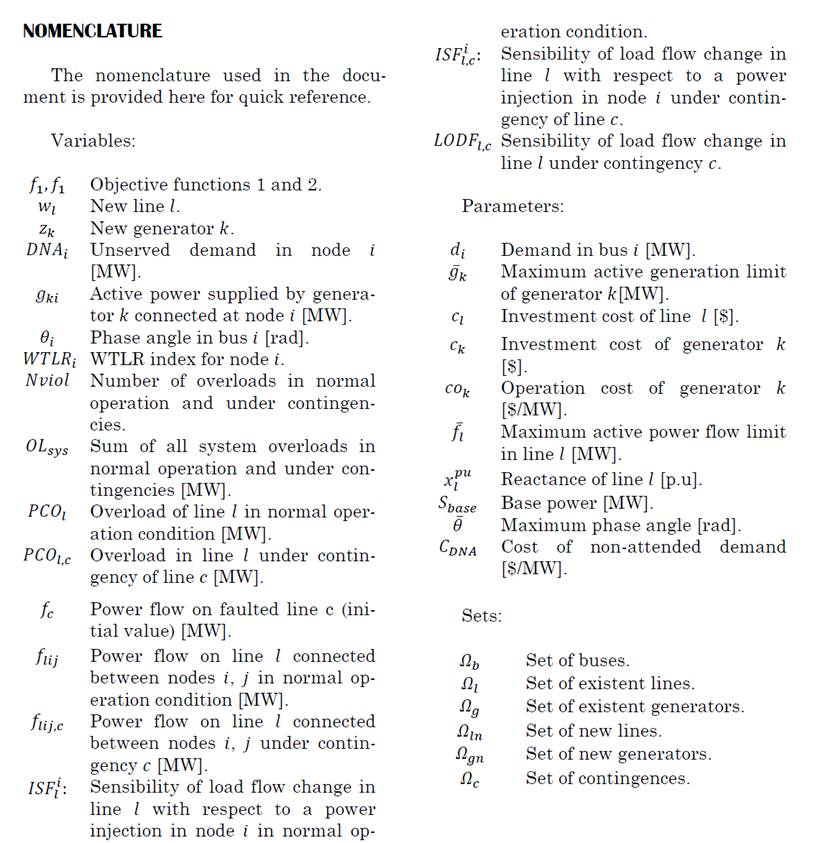
WTLR indexes are given by (3). Note that these indexes are computed once w l and z k are specified. The terms used to compute the WTLR indexes are given by (4)-(10) [26]. They indicate the approximate change in the total overload of the system (in both, normal and contingency states) that would result from a marginal injection of 1MW in a given bus. Since they are based on systems’ injection shift factors, WTLR indexes can take either positive or negative values. The receiving ends of overloaded elements have negative WTLR indexes, which indicates that injecting power into these nodes produces counter flows that relieve the overload. Conversely, the emitting ends of overloaded elements have positive indexes, which indicates that injecting power into these nodes would worsen the overload. To reduce overloads in both normal and under contingency conditions, new elements must be added to the existing transmission network in such way that the magnitudes of the WTLR indexes are reduced. That is to say, if these indexes are equal to zero there are no overloads, neither in normal operation nor under contingencies.
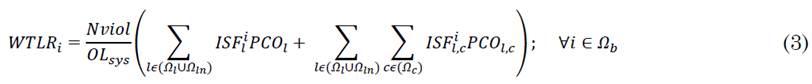
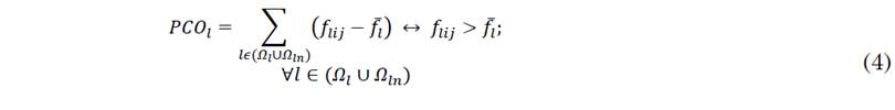


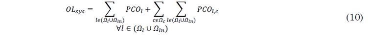
Equations (4) and (5) represent overload limits in lines for normal operation condition. Note that the power flow limits are considered not only for existing lines but also for new ones. Equations (6) and (7) represent overloads in power flow limits of lines under contingency.
In this case, overloads up to 120% of the maximum capacity transmission limit are allowed. This corresponds to a setting selected by the authors; however, any other overload level can be considered. Equation (8) is used to compute the post-contingency power flow of each line for each contingency though the line’s outage distribution factors (LODF). They represent the sensitivity of the change of power flow in each line for each contingency. Constraint (9) represents the injection shift factor (ISF) of each line with respect to each node for each contingency. A Thorough description and details of the computation of LODF and ISF can be consulted in [27] and [28], respectively. It is worth mentioning that power flow limits are taken into account but not enforced within the proposed approach. This is because the proposed expansion plans, as explained in the Method section, represent the best trade-offs between security and costs. If system planners do not have an appropriate budget available, they will have to set up an expansion plan that would eventually result in post-contingency overloads. The set of different expansion plans is represented by an optimal Pareto front, on which the system planner would be able to choose a specific plan according to a given budget. Equation (10) is used for the calculation of the total system overload. Note that overloads are considered in the base case and after contingencies.
2.3 Power balance constraints and limits on other variables
Equation (11) represents the nodal power balance constraint for each node. Equation (12) models the power flows in existing lines, while (13) and (14) represent the power flows of the candidate expansion lines. Equation (15) represents the generation limits of existing generators, while (16) and (17) do the same for new generators. Equation (18) represents maximum limits on phase angles for each bus. Equations (19) and (20) consider the binary nature of the decision variables for lines and generators, respectively. Finally, (21) indicates that the angle of the reference bus must be zero.


3. METHOD
To solve the TNEP problem given by (1)-(21), a multi-objective metaheuristic technique was selected. The implemented algorithm is the so-called NSGA-II [29]. This metaheuristic method was specifically designed for solving multi-objective optimization problems.
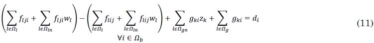
When conflicting objectives are being optimized, there is no single solution to the optimization problem. Instead, a set of solutions represents the best trade-offs between the conflicting objectives. This set of solutions is known as the optimal Pareto front. The solutions within this set are said to be non-dominated, i.e., for a given solution in this front, there is no way of improving one objective without worsening any other. The schematic layout of the NSGA-II procedure is depicted in Fig. 1.
The NSGA-II starts with an initial population of parents P t (N individuals) and creates a descendant population 𝑄 𝑡 (N individuals). The two populations constitute the set 𝑅 𝑡 of size 2N. Subsequently, by non-dominated sorting, the 𝑅 𝑡 population is classified in different Pareto fronts. The new population is generated from configurations of non-dominated fronts. The population is built with the best form of non-dominated solutions (F1), followed by solutions in the second front (F2), and so on.
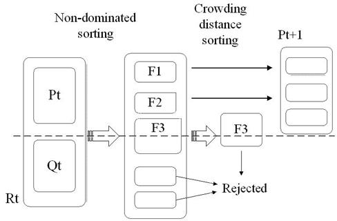
A candidate solution to the TNEP problem is represented by a binary vector that indicates whether a new element must be added to the network. The length of the vector corresponds to the number of candidate lines and generators. If a given position of the vector is zero, it indicates that the corresponding element was not selected in the expansion plan. The flowchart of the implemented NSGA-II is depicted in Fig. 2. Given an initial set of randomly generated candidate solutions, their objective functions are calculated, and the concept of dominance is applied to classify the solutions (non-dominated sorting). The initial population of candidate solutions must go through the stages of tournament selection, crossover and mutation to generate a new set of solutions. Then, a non-dominated sorting of the combined population is carried out as illustrated in Fig. 1. The procedure is repeated until a maximum number of iterations is reached. A detailed description of the implementation the NSGA-II can be consulted in [31] and [32].
4. TESTS AND RESULTS
In order to show the applicability of the proposed approach, several tests were performed with two benchmark power systems: the Gaver system and IEEE 24-bus reliability test system. The data of both systems can be consulted in [33] and [34], respectively. Two scenarios were analyzed for each system. Scenario 1 considers high investment costs in transmission lines, as given in [35]; Scenario 2 considers low investment costs in transmission lines, as presented in [36]. Power flows were computed using Matpower software [37].Three types of generators (10, 20 and 30MW) were considered as additional candidates to be included in TNEP in all load buses. The investment cost of generators was considered to be 1MillionUSD/MW. The results and analysis of the selected test cases are provided below.
4.1 Tests with the Garver system
This system has 6 buses, 6 existing lines, 2 generators and 5 loads that add up to a forecasted demand of 670MW [33]. Bus 6 is not initially connected to the network and its load must be supplied by the expansion plan. All possible combinations of corridors, with maximum 2 new lines per corridor among the 6 buses, are considered.
To adjust the parameters of the NSGA-II, several tests were conducted until the algorithm was able to find high-quality solutions. The best solutions were found using a population of 30 individuals with 100 generations and crossover and mutation rates of 90% and 10%, respectively.
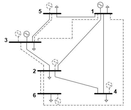
The NSGA-II provides a set of optimal solutions instead of a single one. For Scenario 1 (considering high costs of transmission lines given in [35]), the algorithm found 12 expansion plans marked as dots in Fig. 3. A reduction of the WTLR indexes is related to a more secure system. Note that higher security levels imply higher investment costs and vice versa. It can be noted that the minimum investment that guarantees WTLR indexes approximately equal to zero (no overloads in normal conditions or under contingencies) is 270MUSD$. Higher investments would only marginally improve the security level of the system. This particular solution is illustrated in Fig. 4. The new elements incorporated into the system are indicated with dashed lines.
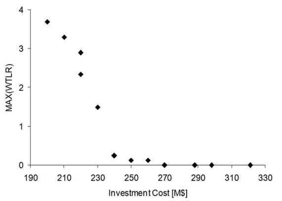
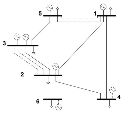
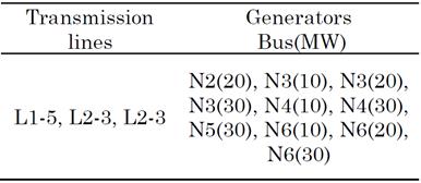
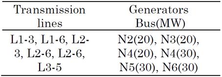
It can be noted in Fig. 4 that no transmission lines are needed to serve the expected demand in Bus 6. Instead, this demand is locally met by new generation. Also, only three new lines are considered in the expansion plan. Details of the expansion plan depicted in Fig.4 are presented in Table 1. The first column indicates the new transmission lines, which are labeled with the number of the nodes they interconnect. The second column indicates the new generators. In this case, the label Bus (MW) indicates the location and size of the generator being proposed. For example, N1(30) means that a generator of 30MW is proposed in Bus 1. Note that several generation units of different capacities can be assigned to a given bus.
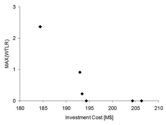
When Scenario 2 is considered (low cost of transmission lines as given in [36]), a new set of optimal solutions is obtained. The Pareto optimal front for Scenario 2 is depicted in Fig. 5. Note that, in this case the minimum investment cost for a secure operation is 195MUSD$. This particular solution is illustrated in Fig 6, in which new elements are drawn as dashed lines. The details of this transmission plan are presented in Table 2.
Source: Authors’ own work.
Fig. 6 Expansion plan with WTLR≈0 and investment cost of 195 MUSD$. Scenario 2.
As expected, more transmission lines are considered in the solution for Scenario 2. In that case, 6 new transmission lines are proposed, in contrast with only 3 for Scenario 1. Furthermore, less generation is needed (see Table 2) and Bus 6 is now interconnected with the rest of the system (see Fig. 6).
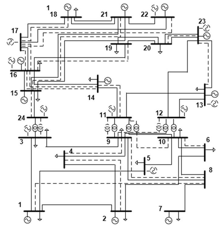
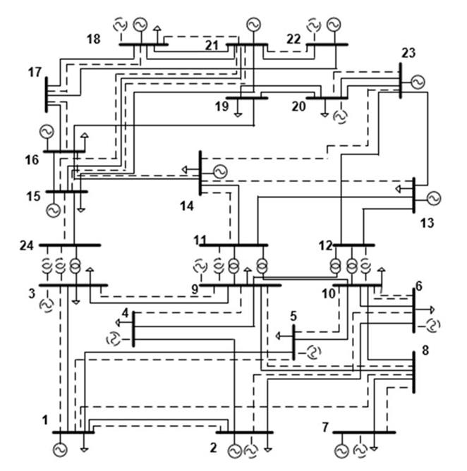
4.2 Tests with the IEEE 24-bus reliability test system
This system comprises 24 buses, 38 lines, and 17 load buses that add up to a future demand of 8,550MW. To carry out the tests with the proposed algorithm, all existing corridors plus 7 more as indicated in [33] were considered. In this system, up to 2 additional lines per corridor can be installed. In addition, the possibility of adding small-scale generation in all load buses was also taken into account. The size and cost of new generators is the same as previously indicated for the Garver system.
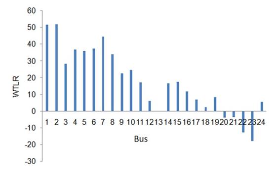
Fig. 7 depicts the initial WTLR indexes computed for this system following the method described in [26]. Note that most of them are far from zero, which indicates that the base case presents overloads after single contingencies.
Several runs of the NSGA-II were performed to adjust its parameters. The best solutions were found with a population of 60 individuals, 100 generations and crossover and mutation rates of 90% and 10%, respectively.
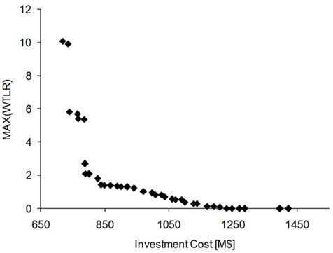
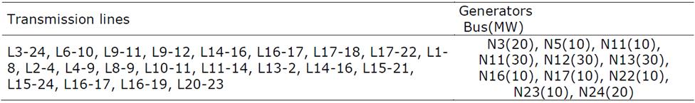
Fig. 8 depicts the optimal Pareto front for Scenario 1. It can be observed that, to guarantee an absence of overloads in normal operating conditions and under contingencies, around 1,200MUSD$ should be invested. Less expensive plans would result in a gradual deterioration of the security levels (higher values of the WTLR indexes). Fig. 9 presents one of the solutions found with the proposed algorithm; it requires an investment cost of 1270MUSD and results in WTLR indexes approximately equal to zero. The details of such investment plan are presented in Table 3. In that case, 21 transmission lines and 11 new generators are proposed in the solution.
Source: Authors.
Fig. 8 Optimal Pareto front for the IEEE 24-bus reliability test system. Scenario 1.
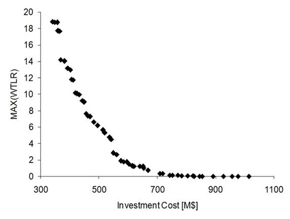
The optimal Pareto front for Scenario 2 is reported in Fig. 10. In that case, guaranteeing network security requires a minimum investment of around 750MUSD$. However, the system planner is provided with a set of optimal solutions to choose according to the budget. It is clear that solutions over 900MUSD$ would be redundant in terms of system security, since they would only marginally reduce WTLR indexes. An expansion plan with an investment cost of 892MUSD is presented in Fig. 10 for illustration purposes, and the details of such plan are included in Table 4.
Source: Authors.
Fig. 10 Optimal Pareto front for the IEEE 24-bus reliability test system. Scenario 2.
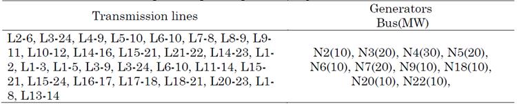
The transmission expansion plan depicted in Fig. 11 requires 29 lines and 10 generators, as indicated in Table 4. As expected, when the cost of transmission lines is lower, more of them are included in the expansion plan.
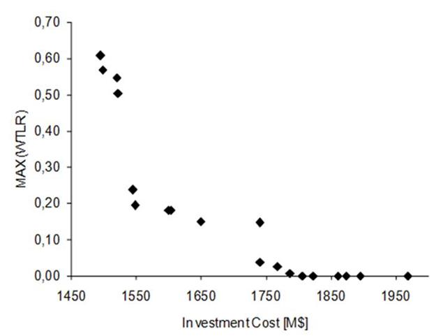
A third scenario was analyzed in this system in order to provide some sensitivity regarding the importance of including small-scale generation in transmission plans. The third scenario considers the costs of transmission lines for Scenario 1 provided in [35] (high investment costs), but does not the inclusion of new generators. The results are summarized in Fig. 12. Note that, in that case, the optimal Pareto front presents more expensive solutions than those reported for Scenarios 1 and 2, (see Figs. 8 and 10). Also, the minimum investment costs that guarantee WTLR indexes approximately equal to zero are around 1,800MUSD$. This represents an increase between 600 and 1,000MUSD$ when compared to the solutions found for Scenarios 1 and 2, respectively.
Source: Authors.
Fig. 12 Optimal Pareto front for the IEEE 24-bus reliability test system. Scenario 3.
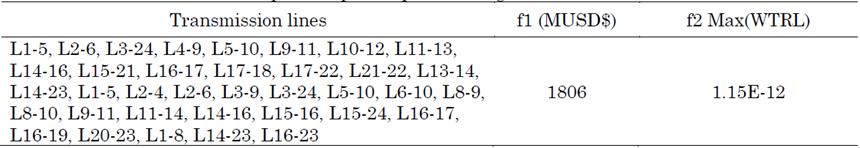
Fig. 13 shows an expansion plan for a solution of 1,806MUSD$ and WTLR indexes approximately zero. In that case, 36 new lines are needed in the system to guarantee security constraints. The new lines are specified in Table 5. Note that only 21 lines were needed in Scenario 1, which considers the same transmission costs but includes small-scale generators.
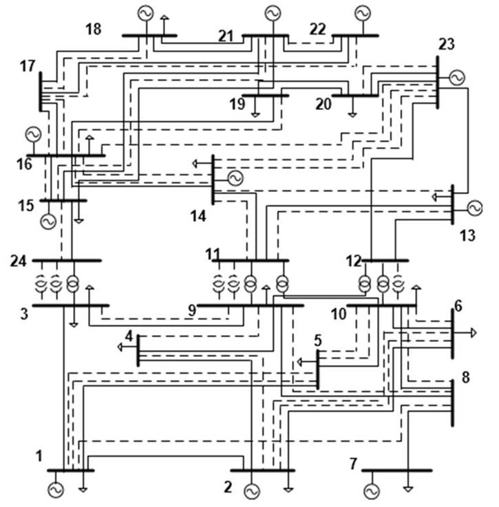
The results allow to conclude that the inclusion of new generators has a positive impact on both security and costs of the expansion plan. This can be explained by the fact that locally supplying part of the demand results in less transmission congestion in both normal operational conditions and under contingencies.
It is worth mentioning that the solutions provided by the proposed method are intended to give alternatives to the system planer regarding new expansion plans. It is the planning engineers who finally decide which solution to implement taking into account budget and regulatory constraints
5. CONCLUSIONS
In this paper an optimization model and solution method were presented to approach the TNEP problem to minimize investment costs and improve network security. The main contribution of this work lies in the use of WTLR nodal indexes, which are expressed as functions of power distribution factors. Such indexes not only measure the level of network security but also identify the most sensitive buses to power injections in terms of post-contingency power flows. In this work, WRLR indexes were used for the double function of diagnosing the system in terms of congestion and guiding the NSGA-II to find better solution proposals. Furthermore, small-scale generators were also included as candidate solutions in expansion plans.
The proposed technique allows to find a set of solutions with different costs and security levels from which the planner can decide depending on the available budget. Several tests on two benchmark power systems showed the applicability and effectiveness of the proposed approach. The inclusion of small-scale generation was found to have a positive effect on transmission expansion plans; it allows to reduce the required number of new lines and contributes to higher security levels. Future work will include a more detailed modeling of generation technologies (such as photovoltaic and wind generation) considered in the expansion plans.

