INTRODUCTION

Hyperspectral images (HSIs) have become a valuable tool for monitoring the Earth surface since they provide a wealth of spectral information compared to traditional RGB images ^[1,2]. HSIs are commonly represented as a 3D data cube, where two dimensions (x,y) correspond to the spatial information and the third one, to the spectral domain (λ). In the 3D cube, each spatial position is represented as a vector, known as a spectral signature, whose values correspond to its intensity in each spectral band. Since the amount of radiation that each material reflects, absorbs, or emits varies according to the wavelength, the spectral signature of each pixel is used as a descriptor in a wide range of applications, such as classification ^[1], target detection ^[2], and spectral unmixing ^[3] among others ^[4-10].

The classification of hyperspectral images can be defined as the process of assigning each pixel to one class. This task is mainly carried out under supervised methods that know some spectral pixel labels which are used in the training stage ^[1]. Then, in the testing process, each unknown pixel is assigned the label of the spectral signature that presents the least spectral difference ^[11].

However, in some applications, the labeled samples are unavailable or difficult to acquire ^[12]. For that reason, unsupervised techniques such as clustering can be an effective alternative because they group a set of similar pixels without previous information of the data. As it is widely known, HSIs are high-dimensional data with large spectral variability and complex structure that make the clustering problem very challenging.

To date, some clustering algorithms have been used for HSIs. Specifically, they can be divided into four groups: (a) centroid-based clustering methods ^[13-15], (b) density-based methods ^[16], ^[17], (c) biological methods ^[18], ^[19], and (d) spectral-based methods ^[8], ^[20]. In general, spectral-based methods have achieved a good and robust performance for spectral images ^[9]. Said methods include two main steps: (i) building an adjacency matrix that describes the relationship between the spectral pixels and, then, (ii) applying centroid-based clustering methods to the Laplacian matrix formed by the adjacency matrix to obtain the clustering results.

Assuming that spectral signatures, which correspond to a land cover class, lie in the same low-dimensional subspace, a known spectral-based method called sparse subspace clustering (SSC) builds the adjacency matrix by expressing each spectral pixel as a linear combination of all spectral signatures of the scene. In addition, such solution is restricted to be sparse, which guarantees that the spectral signatures that correspond to those sparse coefficients belong to the same subspace^[8]. However, in the traditional SSC scheme, only spectral information is used to discriminate the different classes, thus ignoring the rich spatial information contained in the HSIs. To overcome those limitations, different methods have been proposed to incorporate a 2D or 3D spatial regularizer into the SSC algorithm ^[9], ^[21-23]. Said methods use 2D/3D smoothing filters in a reshaped coefficient matrix based on the fact that adjacent coefficients generally belong to the same class. Although those methods have shown good performance for HSIs, when the number of points increases (i.e., the spatial dimension of the image is large), they become computationally intractable ^[22], ^[24].

For that reason, this work proposes to remove some spectral pixels from the image in order to reduce the number of points to classify. Consequently, the computational time of the clustering task is reduced. Afterward, the clustering results of the incomplete pixels are assigned using a kind of filter that selects the predominant label in a given neighborhood. Specifically, this work proposes two schemes to remove some spectral pixels. The first one is based on spatial blue noise coding ^[22,25], and it allows uniform elimination in the spatial dimensions of the scene, avoiding clusters of removed pixels, which are properties desired in the filtering step. The second one is a sub-sampling scheme that eliminates every two contiguous pixels preserving the spatial structure of the images, which allows the use of SSC-based methods that employ the spatial information to improve the clustering result ^[21], ^[26]. The performance of the spectral image clustering framework proposed in this study is evaluated using three datasets, and a similar accuracy is obtained when up to 50% of the pixels are removed compared with the full data using the proposed designs. In addition, the proposed scheme is up to 7.9 times faster classifying the data sets compared to the full data sets.

2. SPARSE SUBSPACE CLUSTERING FOR HYPERSPECTRAL IMAGES

Let F∈R^L×MN be a hyperspectral image reorganized as F=[f ₍₁₎ ,…,f _(MN) ], where M and N represent the spatial dimensions, L stands for the number of spectral bands, and f _(k) ∈ R ^L denotes the spectral signature of the k -th pixel. The SSC method assumes that the HSIs lie in the union of n low-dimensional subspaces such that each subspace corresponds to a certain land-cover class ^[26]. In order to group spectral pixels, SSC assumes that each spectral signature f _(k) that corresponds to a specific land-cover class belongs to the same independent subspace ^[9]. Specifically, first, the SSC builds a sparse similarity matrix, which describes the relationships between pixels exploiting the fact that each spectral signature is represented as a linear or affine combination of few pixels in the same subspace ^[8]. This affinity matrix is built using the coefficient matrix C ∈ R^MN×MN obtained from the sparse optimization problem, which is modeled as follows (1):

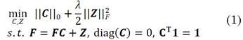
where, -norm is the number of nonzero elements of C; Z , the error matrix; and λ, a regularization parameter for the sparsity coefficient and noise level trade-off. The constraint diag (C)=0 is used to eliminate the trivial ambiguity where a point is represented by itself, and the constraint C ^T 1=1 ensures that it can work even in case of affine subspaces ^[8], ^[24]. After solving (1), the k-th column of C , which corresponds to a data point f _(k) that lies in a d _i dimensional subspace S _i , is expected to have only d _i non-zero elements. However, since ℓ₀-norm is an NP-hard problem, the relaxed -norm is usually adopted to relax the problem as (2):

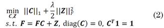
where, the -norm promotes sparsity, i.e., each spectral signature is represented by few pixels ^[8]. This formulation can be efficiently solved using the alternating direction method of multipliers (ADMM) with a computational complexity O(L(MN) ² ) ^[27]. After solving (2), each column of C is normalized to better deal with different norms of the spectral signatures as c _j =c _j /||c _j ||∞. Subsequently, C is used to construct the non-negative similarity matrix W as (3):

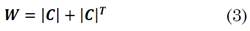
where, W _i,j represents the similarity between the i-th and j-th pixels. Finally, to obtain the segmentation of the data into different subspaces, a weighted graph G=(ν,ε,W) is built, where ν denotes the set of NM nodes of the graph that correspond to NM pixels of the image; ε ⊆ ν×ν, the set of edges between the node; and W ∈ R ^MN×MN , the weights of the edges. Then, the data is clustered by applying spectral clustering methods ^[8,28] over the graph G which, naively implemented, has a computational complexity O((MN) ³ ) ^[8].

3. SPARSE SUBSPACE CLUSTERING FOR HYPERSPECTRAL IMAGES WITH INCOMPLETE PIXELS

Note that this sparse representation builds the C matrix using only spectral information, i.e., the sparse representation of the k-th pixel is the same regardless of its spatial position. Therefore, considering that land-cover materials are distributed homogeneously (i.e., contiguous pixels in a spectral image generally belong to the same material), different constraints have been applied to C in order to incorporate the spatial information of the scene ^[9], ^[21]-[23], ^[26], ^[29]. Specifically, different smoothing filters are applied at each iteration of the ADMM algorithm to a reshaped version of the C matrix in order to obtain the same value in a neighborhood of pixels ^[9], ^[21]-[23]. Furthermore, the use of smoothing operators on the image has been explored for SSC ^[23], ^[29]. Although said method has shown good results in non-supervised classification tasks, when the spatial resolution of those images increases, they become computationally intractable ^[24].

For that reason, we propose to remove certain pixels from the image before solving step (2) and the spectral clustering method in order to reduce the computational time of those steps. Mathematically, the incomplete image can be represented as (4):

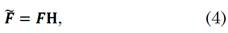
where, F ̃ is the incomplete image, and H ∈ {0,1} ^MN×P is the selecting matrix that has only one non-zero value per row, with P as the number of preserved pixels. Therefore, the SSC model is applied to obtain the clustering results for those pixels. This segmentation can be represented in s ∈ R^P, which is a vector with the labels of the preserved pixels. In order to obtain the incomplete labels, let s ̂= Hs be a vector where the missing positions are present. Then, this vector is reorganized in a matrix S ∈ R ^M×N (see Fig. 1), where the incomplete labels are obtained applying a kind of filter that selects the predominant label in a given window; in this case, of a 3 ×3 size. Specifically, when χ={1, ...,ı} denotes the set of ı class labels, those missing values are given by (5):

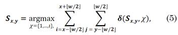
where w=3 is the size of the window; ⌊.⌋, the floor function; and δ, the Kronecker delta function, which is 1 if the arguments are equal and 0 otherwise.

Fig. 1 represents the step-by-step of the proposed method and Algorithm 1 summarizes the computations described above. Note that the quality of the proposed methodology mainly depends on the structure of matrix H. For that reason, the two following sub-sections propose different strategies to design selecting matrix H in an efficient way.

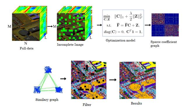
Source: Authors’ own work.

Fig. 1 Visual step-by-step process of the sparse subspace clustering for hyperspectral images with incomplete pixels showing the full data in a 3D structure 

Algorithm 1: Spectral Subspace Clustering for incomplete hyperspectral image

Input: F, n, λ, H, p

Output: Segmentation of the data S

3.1 Design of the Selecting Matrix Based on Spatial Blue Noise Coding

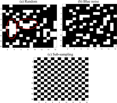
An important design parameter of the selection matrix is the number of pixels that will be removed. Therefore, let ζ _r be the preservation ratio defined as (6):

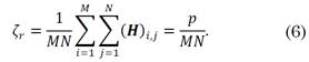
For instance, ζ _r = 0.2 means that 20% of the pixels would be preserved and 80% of the pixels would be removed after applying (4). A conventional selection matrix uses random entries; however, random binary codes tend to form clusters. Figure 2 (a) shows an example of a random matrix with ζ _r = 0.75, where matrix H is represented as an M × N matrix where white spaces mark the pixels to remove, and black represents the pixels to keep. Note that the random matrix tends to form clusters, which leads to a negative impact when the non-labeled pixels in the incomplete image are assigned using the strategy presented in Section 3. For that reason, a blue noise pixel distribution is used in order to reduce clusters and achieve uniform selected pixels, as shown in Fig. 2. (b) ^[25].

Source: Authors’ own work.

Fig. 2 Visual representation of selecting matrix H for (a) random distribution and (b) blue noise distribution with ζ _r = 0.75, and c) sub-sampling with ζ _r = 0.5 

3.2 Design of the Selecting Matrix-Based Sub-sampling

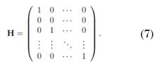
The random and spatial blue noise criteria to remove pixels do not preserve the spatial distribution of the scene after the reorganization in (4) because more rows than columns, or vice versa, can be eliminated. Therefore, SSC-based methods that incorporate the spatial information cannot be directly applied to F̃. For that reason, a sub-sampling scheme that eliminates every two contiguous pixels and preserved the spatial structure of the images is proposed. Specifically, matrix H has the structure (7).

4. SIMULATIONS AND RESULTS

In this section, the performance of the proposed hyperspectral image clustering framework is evaluated. The clustering result of applying Algorithm 1 to the incomplete image is denoted as IP. The spectral Indian Pines dataset and two regions of Pavia University data set were used for these experiments. The results presented here are the average of 10 trial runs. Overall accuracy (Acc_O), average accuracy (Acc_A), and Kappa coefficients were used as quantitative performance metrics. In the tables, the metric used for each land cover class is Accuracy. All the simulations were implemented in Matlab 2017a on an Intel Core i7 3.41-Ghz CPU with 32 GB of RAM. In all the tables, the optimal value of each row is shown in bold.

4.1 Spectral image datasets

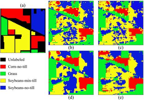
The Indian Pines hyperspectral data set, sensed by the AVIRIS sensor, has 145 × 145 pixels and 224 spectral bands ^[30]. A total of 20 water absorption and noisy bands were removed, thus leaving 200 spectral features for the experiments. A known sub-image of the Indian Pines data set was used in the test; its spatial dimensions are 70 × 70 pixels, and it includes four main-land cover classes: corn-no-till, grass, soybeans-minimum-till, and soybeans-no-till ^[9].

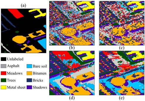
The second scene, of Pavia University, was acquired by the Reflective Optics System Imaging Spectrometer (ROSIS) airborne sensor over an urban area of Pavia, Northern Italy. The size of the image is 610 × 340 pixels and 103 spectral bands ^[9]. For the tests, the authors selected a typical area of a size of 140 x 80 pixels containing eight main land-cover classes: asphalt, meadows, trees, metal sheet, bare soil, bitumen, bricks, and shadows. Furthermore, a different region of ROSIS Pavia University data set was also used; its size is 64 × 64 pixels, and it contains four land-cover classes: asphalt, meadows, trees, and bricks.

The number of classes for each data set was manually fixed as an input for Algorithm 1. Additionally, parameter λ was chosen applying the formulation in ^[9] as (8):

where, γ is a parameter that directly depends on the spectral image that is used and β is a tunable parameter that was fixed for all the experiments at β=1000.

4.2 Quality of classification results vs number of eliminated pixels

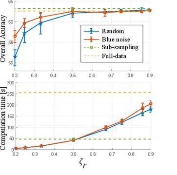
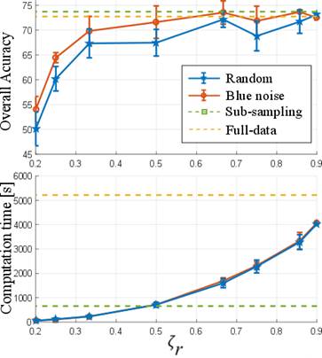
The first test was performed to show the quality of the results and the computational time using the number of eliminated pixels by means of the preservation ratio (ζ _r ). For that purpose, the proposed methods were compared with random elimination and the complete image. The Indian Pines and Pavia University data tests were used in this test. Figure 3 and 4 show the general accuracy and the computational time obtained with the different configurations for the two data sets, respectively. Note that, in the sub-sampling method, the preservation ratio is fixed at ζ _r = 0.5 and, with the full image, it is ζ _r = 1. It can be observed that, when the number of preserved pixels increases, the quality of the classification by the designed and randomized elimination schemes improves. However, the designed blue noise scheme outperforms the random selection matrix with ζ _r ≤0.5 for both data sets. In addition, the proposed methods maintain a performance comparable to the full data when more than half of the pixels are conserved. Fig. 3 and 4 also show the time spent applying different preservation ratios and a drastic increase in computational time as the number of removed pixels decreases.

Source: Authors’ own work.

Fig. 3 Preservation ratio versus (top) overall accuracy of the clustering result and (bottom) computational time for the Indian Pines data set 

Source: Authors’ own work.

Fig. 4 Preservation ratio versus (top) overall accuracy of the clustering result and (bottom) computational time for the Pavia University data set 

4.3 Advantages of the Sub-sampling scheme

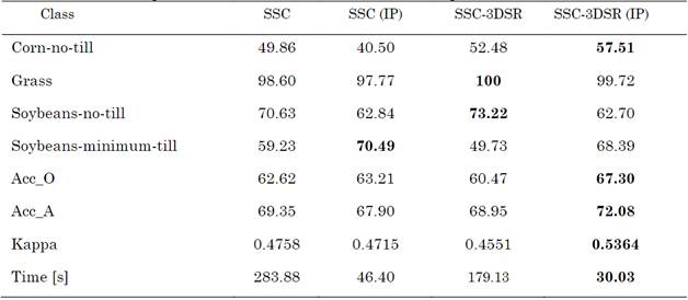
The second test shows the advantages of the sub-sampling method because SSC with spatial regularizer (SSC-SR) algorithms can be used. Therefore, the SSC with a 3D spatial regularizer (SSC-3DSR) was employed for this test ^[22]. Figure 5 and Table 1 show the detailed results of the classification and computational time, respectively, for the Indian Pines data set. Note that the SSC-3DSR and SSC-3DSR (IP) obtained a better clustering accuracy. In addition, the proposed approach obtained clustering results comparable to the classification of the full data by the SSC and SSC-3DSR methods. Nevertheless, the proposed method reduces the computational time by 83.65% and 83.23% compared to SSC and SSC-3DSR, respectively.

Source: Authors’ own work.

Fig. 5 Visual clustering results on AVIRIS Indian Pines image: (a) ground truth, (b) SSC, (c) SSC (IP), (d) SSC-3DSR, and (e) SSC-3DSR (IP) 

Table 1 Clustering results for the AVIRIS Indian Pines Image 

Source: Authors’ own work.

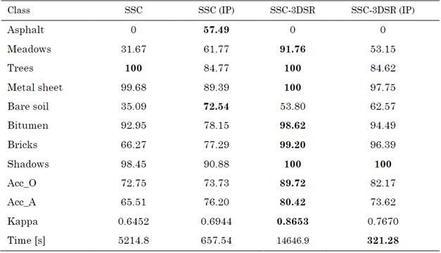
Furthermore, Figure 6 and Table 2 show the visual and numerical results of the first region of the Pavia University dataset in terms of classification accuracy. For this dataset, the best result is achieved by the SSC-3DSR without the proposed subsampling method. Moreover, the proposed scheme provides the shortest classification time, thus maintaining a good performance. Specifically, it solved the clustering problem 6.11 times faster than the other methods.

Source: Authors’ own work.

Fig. 6 Visual clustering results on ROSIS Pavia University image: (a) ground truth, (b) SSC, (c) SSC (IP), (d) SSC-3DSR, and (e) SSC-3DSR (IP) 

Table 2 Clustering results for the ROSIS Pavia University image 

Source: Authors’ own work.

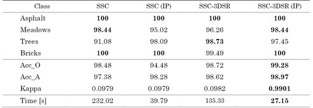
Finally, the classification performance achieved for the other region of the Pavia University dataset is shown in Fig. 7, and the quantitative results are presented in Table 3. Note that the quality is preserved, but our method is 5 times faster for this subregion of Pavia University.

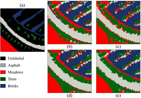
Source: Authors’ own work.

Fig. 7 Visual clustering results for a region of Pavia University image: (a) ground truth, (b) SSC, (c) SSC (IP), (d) SSC-3DSR, and (e) SSC-3DSR (IP) 

Table 3 Clustering results for a region of Pavia University image 

Source: Authors’ own work.

5. CONCLUSIONS

A method to reduce the computational time of sparse subspace clustering for hyperspectral images was proposed in this work. Such scheme is based on the fact that some spectral pixels can be omitted in the clustering steps. Therefore, the clustering of the removed pixels is completed using a special filter that selects the most frequent value in a given neighborhood. Specifically, this work proposed two schemes to remove pixels. One is based on spatial uniform blue noise coding, and the other is a sub-sampling of every two pixels that preserves the spatial structure of the scene. In general, the results for three different datasets show that the proposed clustering achieves similar accuracy, but it is up to 7.9 times faster than the other methods. However, removing some pixels can sharply reduce classification accuracy in some images, especially when there are few pixels per class. Therefore, future work includes grouping pixels according to the spatial structure of the scene instead of eliminating them.