


 English (pdf)
 Article in xml format
 Article references
 Send this article by e-mail
 Cited by SciELO
  Cited by Google
  Similars in
SciELO
Similars in
SciELO  Similars in Google
 Permalink
1. INTRODUCTION
In modern agricultural systems, pipe network systems are completely based on replacing open channels with pressurized networks. These systems enable a more efficient transmission and distribution of water to farmlands and plots by reducing evaporation and seepage losses. In these types of pressurized networks, different pipelines are employed in the plots and sub-plots designated for agricultural purposes. The materials used to manufacture these pipeline systems are chosen for their long lifespan and low purchase and maintenance costs. Designing a network often requires optimally selecting the different diameters for the pipes in the network. An optimal design involves a cost-effective propagation of a given fluid to the desired area at the required head and flow rate [1].
The flow dynamics occurring during water transmission through a network are entirely determined by various fundamental physical laws. To design an optimal pipe for a network, two methodologies are usually employed: the analysis approach and the design approach.
Selecting an optimal diameter for a pipe network entails various constraints, such as an allowable pressure drop or a required flow rate, depending on the nature of the fluid composition and the materials used to design the pipes. This type of optimal pipe design is referred to as the design methodology, and it serves as the foundation for deducing empirical formulas to determine the required diameter for any type of pressurized network [2].
An estimated pipe diameter can be classified as optimal if it minimizes the life cycle cost of the piping network. Capital expenditures and recurring costs associated with the operation and maintenance of a network system are analyzed considering time and money as primary factors. When selecting a pipe diameter for a given network, there exists a trade-off between large and small pipe diameters depending on various criteria. A large diameter implies higher capital expenditures in the initial state but lower recurring costs in maintenance and operation, as it leads to minimum head losses and a subsequent reduction in energy consumption. In contrast, a small diameter entails a lower initial purchase cost but higher recurring costs due to a considerable increase in pressure head losses resulting in higher energy consumption. Considering the selection criteria mentioned above, the optimal diameter for a network is chosen based on the hydraulic and economic analysis of the pipe network.
Depending on the nature of the flow, fluid flows are generally classified into two categories: gravity flow and pressurized flow. In fluid flow dynamics, a pressurized fluid flow involves a number of physical variables. These variables usually act as constraints during the flow of a fluid through the pipeline and play a role in determining the optimal diameter for a network [2].
Several authors have proposed empirical equations to estimate the optimal pipe diameter for a particular pipe network. For instance, an empirical equation obtained for the design of an optimal pipe size for PVC and HDPE materials is discussed in [3].
Moreover, various empirical and mathematical models employed to select an economical pipe based on different pipe diameters for six distinct materials are elaborated on in [1].
These models were further developed to calculate fixed and operating costs depending on various physical variables such as flow rate, electricity cost, and length. In [4], an optimal pipe diameter equation was designed using a nomograph. This formula considers both hydraulic and economic properties with two cost factors: piping and pumping costs. The authors of [5] describe a preliminary pipe sizing technique that involves quick size estimation for normal pressure fluid flow.
A set of alternatives to the API RP 14E equation are presented in [6], as well as a comparison between the calculated and experimentally determined erosion velocity values using different models.
A velocity known as “economic design velocity” was selected across the entire pipeline network. The authors of [7] suggested this notion of constant velocity, which leads to the lowest total annual costs, for the design of a network comprising the mains and the branches for three different markets: the Lebanese, American, and Indian markets. In [8], Smit proposed a formula to estimate the optimal diameter based on annual pumping hours and illustrated the multiple pipe selection processes under South African conditions. In [9], Diniz and Souza presented four explicit equations to calculate the friction factor for all the flow regime conditions of the Moody diagram without employing iterative procedures. In [10], Zocoler et al. designed a model to determine the economic velocity and diameter of fluid flows using the modeled diameter equation obtained by means of the Swamee’s friction factor in order to minimize total annual costs.
Furthermore, a method for the design of an optimal pipe, considering a limit on the velocity factor of the fluid flow, was proposed in [11] because flow velocity is a primary factor that affects the nature of the flow through the pipes. In [12], the life cycle analysis technique was performed on six different pipe materials used for water and wastewater applications, and the results were compared in terms of global warming potential across the four phases of the life cycle analysis. In [13], the concept of genetic algorithm was applied to a water company located in South Africa to determine the optimal pipe diameter by means of an application called GAPOP. In [14], the finite element model and the life-cycle cost analysis technique were implemented to formulate the optimization and analysis of complex networks. In [15], the genetic algorithm technique was compared to the complete enumeration and nonlinear programming techniques for pipe network optimization. In [16], an approach based on computer programming was applied to select the optimal pipe diameter by incorporating various operating and capital costs. In [17], the authors addressed different methods for measuring spring discharges. They also discussed the various applications in which these methods can be used. In [18], the long-life expectancy of PVC pipes was thoroughly reviewed. Such paper summarizes the results of multiple tests conducted by Utah State University and several researchers to examine the expected life of PVC pipes.
Based on this literature review, this study seeks to model an optimal pipe design for the network at the Hamelmalo Agricultural College (HAC) farm, which consists of the mains and various sub-mains. It begins with the design of optimal pipe sizes using the mathematical model proposed by A. Sonowal et al. [1], which is part of the process of the recommended life-cycle cost analysis. Afterwards, the pipe sizes are estimated using different empirical formulations depending on the various physical variables involved in the flow. This study aims to compare the pipe sizes designed using the empirical formulas with those provided by the standard technique and find the best-fit model considering friction losses, total cost analysis, and certain statistical indicators.
The rest of this paper is structured as follows. Section 2 presents a detailed description of the methods and materials employed to collect the experimental data. It also summarizes the methodologies implemented to determine the pipe diameter using various empirical equations. Section 3 compares the different models considering a cost analysis, friction losses, and certain statistical indicators. Section 4 draws the conclusions based on the comparison of the methods. Section 5 contains the acknowledgements. Finally, Section 6 lists the references used in this paper.
2. MATERIALS AND METHODS
2.1 Experimental data collection
The network at the Hamelmalo Agricultural College (HAC) farm in the Anseba region of Eritrea, for which optimal pipe sizes were to be designed, was chosen as the case study.
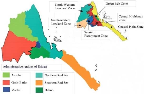
Figure 1 shows the various administrative regions of Eritrea. HAC is located in the Anseba region, one of the administrative regions lying at 15°52’35” N latitude and 38°27’45” E longitude, with an elevation of 1264 m above sea level and a semi-arid climate [19].
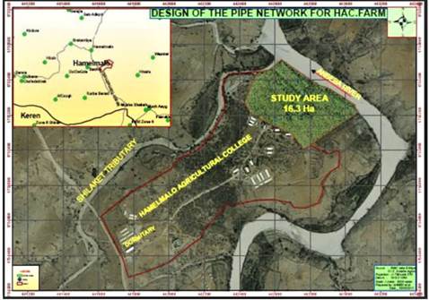
HAC is bordered on the north by the Anseba river and on the north-west by Shilaket, which is a tributary of the Anseba river. The farm area is estimated to be about 16.3 hectares, as shown in Figure 2. In addition, it is covered by brown sandy loam soil with sand, slit, and clay deposits of different compositions [20].
The farm is divided into several sub-plots; each categorized according to the college’s various departments. The research studies of each department are generally conducted in their respective sub-plots. The existing pipe network at the HAC farm is linear. The water for the network basically comes from two wells that draw water from the Anseba River.
Although the network is primarily supplied by one well, which discharges water at a rate of 18 L/s, the other well, which releases water at a rate of 8.3 L/s [11], serves as a redundant in times of scarcity, as shown in Figure 3 taken from [20].
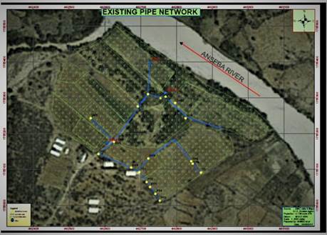
Source: [20].
Figure 3 Satellite image of the hydraulic pipe network at Hamelmalo Agricultural College
The existing pipe network at the HAC farm consists of a mainline, along with numerous minor fittings, in order to deliver water to the different sub-sections of the farm. Each plot is assigned a specific crop type. The cropping pattern includes fruits such as mango, papaya, and oranges, as well as forage crops like alfalfa. Potatoes, tomatoes, and cereals such as sorghum are among the vegetable crops grown. Crops are both rain-fed and irrigated. The pipes installed in the farm are mostly made of Galvanized Iron (GI), and just a few are made of Polyvinyl Chloride (PVC). Since this study aims to design an optimal diameter for the chosen pressurized network, PVC was selected, over other materials, for the pipe design because of its significant features and widespread use in the market.
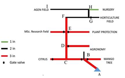
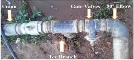
A hydraulic analysis chart was designed in order to determine the exact length of the network’s pipe links (as shown in Figure 4 and Figure 5), as well as of the study’s sample minor fittings (as shown in Figure 6) [11]. Regarding the fluid chosen for this study, properties such as its viscosity, temperature, and volumetric flow rate for the existing network were also estimated. The triangle in the figures represents the pump, which acts as the source. Figure 4 illustrates the network’s various links, whereas Figure 5 depicts the different college’s departments.
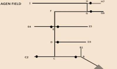
Source: [11].
Figure 4 Hydraulic analysis chart of the network at the Hamelmalo Agricultural College farm
Source: [11].
Figure 5 Hydraulic analysis chart of the existing network at the Hamelmalo Agricultural College farm considering the different college’s departments
Source: [11].
Figure 6 Sample of the minor fittings available in a section of the network available at the Hamelmalo Agricultural College farm
PVC is usually the material chosen for pipe networks due to its widespread use and enormous benefits over other materials. Compared to other pipe materials, it has a good tensile strength. PVC pipes are generally resistant to corrosion and malleable, which makes them much easier to be employed in a variety of applications. Since they have a high degree of freedom combined with malleable properties, they can be designed in different fashions.
In comparison to pipes made of other materials, these pipes are highly resistant to cracks and fractures. In addition, because they are normally inert to chemicals, they can be manufactured for different types of fluid flows. There is often a significant difference in frictional head losses when fluids flow through PVC pipes versus pipes made of other materials. Frictional head losses in PVC pipes are re considerably lower, making them ideal for fluid flows in irrigation. These pipes have a life expectancy ranging from 50 to 70 years and can be used at a relatively high temperature such as 60 °C [21], [22].
Considering the features mentioned above, PVC was the material chosen to design the optimal diameter for the network under analysis. The relative roughness, friction factor, and friction head loss of the fluid flow for the network were estimated based on this assumption.
An electronic theodolite and a Garmin Oregon 550 GPS were used to survey the farm where the network is located and to estimate its elevation. Water discharge was measured using a graduated measuring cylinder and a stopwatch. The bucket-and-stopwatch method was implemented to calculate the discharge in the pipes, as discussed in [17]. Since temperature varies depending on the system’s viscosity and density, the nominal temperature of the flow was estimated using a thermometer. A submersible pump was employed to pump water from the well to the network at a rate of 18 L/s.
The efficiency of the power units was assumed to be 75 %. The brake power and Water Power (WP) energy of the submersible pump were estimated to be 24.61 kW and 13.76 kW, respectively. The entire network was divided into 15 links in order to design the optimal pipe diameter for the network based on the estimated discharge. The length of the different links for the pipes was determined using an odometer and a tape arrangement. A number of minor fittings were used to deliver water to the sub-plots in the existing network.
As suggested in [23], [24] as a requirement to design an optimal pipe diameter for a specific pressurized network, minor local losses were assumed to be above 10 % of the total estimated major friction losses in the corresponding 15 links. Major friction loss is considered a predominant factor that affects water flow through the pipes. A number of empirical models have been proposed by several authors to determine the major friction loss occurring through the pipes. The implicit Colebrook’s equation is a model empirical equation that was developed during the early stages to estimate the friction coefficient in the Darcy-Weisbach equation. The Darcy-Weisbach equation is given by (1).
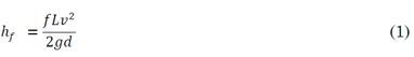
In this equation, h f is the friction head loss in m; f, the friction co-efficient, which is a function of the two variables, i.e., the Reynolds number (Re) and the relative roughness of the pipe (ɛ); L, the length of the section of the pipe in m; v, the average flow velocity in the pipe in m/s; g the gravity component in m/s2; and d, the hydraulic diameter of the pipe in m.
Due to the implicit nature of the friction coefficient (f), it is given by (2), as proposed by Colebrook.
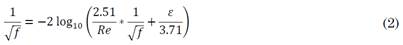
In this equation, f denotes the friction coefficient; Re, the Reynolds number; and ε, the relative roughness of the pipe’s inner surface.
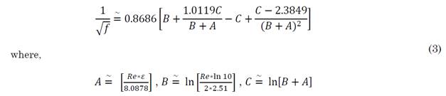
The Hazen-Williams equation became popular in the industrial sectors, as opposed to the Darcy-Weisbach equation, although, according to several authors, the Hazen-Williams equation has a number of limitations. Various empirical models have been proposed to overcome the implicit nature of Colebrook’s equation. These equations were usually proposed under a number of constraints depending on the nature of the fluid, the medium, and the nature of the flow, as well as the industries in which the process occurs. In this study, the friction factor was calculated using the shifted Lambert W function. The equation proposed in [25] estimates the friction factor more accurately, with a relative error of less than 0.0096 %. The implicit Colebrook-White equation has been stated here in terms of the Wright ω function. Given the huge importance and applications of the Lambert W function in various fields, the authors developed the equation presented below, which was applied to the case study in order to compute the friction factor correctly (compared to that of Colebrook’s equation). The explicit equation used to determine the friction factor is given by (3).
2.2 Methodologies to determine the optimal pipe diameter
Optimal economic pipe size selection for the delivery of a fluid to various sub-plots is generally based on the principles of engineering economics [2]. This process usually involves a series of steps to determine the optimal diameter for a given network depending on a number of constraints.
2.3 The Life-Cycle Cost Analysis (LCCA) model
As suggested in [26], Life-Cycle Cost Analysis (LCCA) is often considered the standard recommended model used to estimate the optimal diameter for any given scenario. During the diameter design, the annual installation and associated annual operating costs are analyzed. These fixed and operating costs depend, in turn, on a number of variable factors that normally affect the design of the optimal diameter. In the LCCA model, the break-even analysis theory is applied to any pressurized flow system in which there exists a trade-off between costs and pipe sizes. This model accounts for the overall lifetime costs: from the initial purchase cost of each pipe in a network to their installation, operation, and maintenance costs.
The procedure to determine the optimal pipe size using the LCCA method is briefly explained below. Based on the knowledge of the fluid flow rate, the different pipe sizes available in the market are chosen on a trial basis. The various fluid parameters, such as flow rate, fluid properties, pipe length and composition, friction factor, Reynolds number, and friction head loss are estimated. The corresponding minor and elevation losses that contribute to the total head losses are also determined. The efficiency of the power units usually ranges from 75 % to 90 % [1]. The total annual operating energy is calculated based on the system’s running hours.
The recommended mathematical economic model that is part of the standard LCCA method adopted in [1] was used in this study to estimate the optimal pipe diameter. The principle involves the estimation of optimum diameter which involves two major cost analysis for any pipe considered. Primarily, it’s the fixed cost which involves the product of present current amount of the pipes, the capital recovery factor for n periods and the length L for a given pipe of diameter d. The second is the operation and maintenance cost which depends on a number of variables. The total costs of any optimal pipe diameter selected are the sum of the fixed and operating costs. Depending on the length (L) and the volumetric flow rate (Q), the different diameters available in the market and retail shops are collected and compared, and the pipe diameter with the lowest total costs is chosen as the optimal pipe diameter. The fixed costs of a pipe of length L are given by (4) [1].
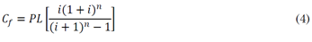
In this equation, C f denotes the annual fixed costs in Nakfa/year; P, the price per unit length of the pipe in Nakfa/m; i, the interest rate in fraction, which equals 0.3; n, the lifespan of the pipe in years, which is assumed to be 50 years; and L, the length of the pipe in m.
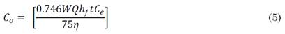
The operating costs during water flow are determined by multiple variables, including pipe diameter, flow discharge, friction head loss, pump usage in hour/year, cost of electricity in Nakfa/kWh, and engine’s efficiency. The annual operating costs to overcome friction during water flow are given by (5).
By substituting the value of the friction head loss coefficient in (5), the annual operation and maintenance costs of the chosen pipe are given by (6) [1].
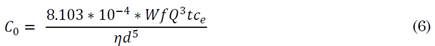
In this equation, C 0 represents the annual operating costs in Nakfa/year; W, the unit weight of water in kg/m3; f, the friction factor; Q, the discharge in m3/s; t, pump usage in hour/year, which, in this case study, was estimated to be 2,920 hour/year; c e , the cost of electricity in Nakfa/kWh, which was found to be 2.65 Nakfa/ kWh; η, the efficiency of the power unit in percentage, which is assumed to be 75 %; d, the pipe diameter in m; and h f , the friction head loss in m.
From the equations mentioned above, the total costs of the pipes are the sum of (c f ) and (c 0 ) and are given by (7) [1]. Hence
In this equation, c t denotes the total costs per unit length of the pipe in Nakfa/year.
This is the recommended mathematical model equation that is part of the standard LCCA method employed to estimate the optimal economic pipe diameter. The overall process of determining the optimal pipe model involves capital expenditures and operation and maintenance costs, which are given by (8).

Capital expenditures comprise the cost of the pipes, power units, and pipe laying, whereas operation and maintenance costs include the energy charges during the flow process. Since this process affects the horsepower of the pump, it depends on a number of parameters. By minimizing the present value in (8), the optimal economic pipe diameter is estimated [1].
Since the process in this case study only involves selecting the optimal pipe diameter for a network based on the mathematical model proposed in [1] and given by (7), it merely focuses on the two major costs of the pipes: fixed costs and operating costs, which are given by (4) and (6), respectively. This selection of the optimal pipe for a specific application from all the available pipes is part of the overall LCCA process defined by (8). This paper discusses in detail how to choose the optimal economic diameter for a network using the mathematical model given by (7) and proposed in [1].
2.4 Bresse’s model
One of the earliest empirical equations proposed to design pipes was developed by Jacques Antoine Charles Bresse, a French professor and applied mathematician [10]. This equation was intended for continuous operating and minimal costs for a given volumetric flow rate through the pipes. As suggested in [27], it was based on Dupit’s equation, which is given by (9).

In this equation, D denotes the pipe diameter in m; k, the constant; and Q, the discharge in m3/s. The value of k is often assumed to be 1.60 and depends on a number of variables, such as the cost of coal, the pipes, and their operation and maintenance services. Bresse further proposed a value of 1.50 when this equation was adapted. In order to estimate the optimal pipe diameter, this case study considered the value of k to be 1.50, as adapted by Bresse. Equation (9) is widely used by hydraulic designers when it comes to small distribution and continuous operation networks [10], [27].
2.5 Bedjaoui-Achour-Bouziane model (model proposed by Bedjaoui et al.)
Bedjaoui, Achour, and Bouziane proposed an empirical equation to select an optimal economical pipe diameter. Such selection was based on the investment costs in the pipes, as well as the operating costs associated with them. The objective was to minimize both costs in order to find an empirical optimal diameter for their study. They obtained the empirical formula through a series of experiments conducted on asbestos cement, PVC, and PEHD pipes with varying operating pressures and hours of operation. From these experiments, they developed an empirical equation to design an optimal diameter, as given by (10) and as proposed in [3].
In this equation, D is the pipe diameter in m; and Q, the discharge in m3/s.
2.6 Jack’s Cube model
Jack N. Adams, a process engineering supervisor, proposed a rule of correlation as a rule of thumb for calculating optimal pipe diameters. The proposed empirical equation serves as a starting point for optimal pipe sizing and can be applied under a normal pressure constraint.
The method used to determine an optimal diameter is known as Jack’s Cube method for pipe sizing. The equation is generally employed in situations where the fluid under consideration should not be too viscous and contain any slurries or crystals. The regression analysis of the cubic expression simplifies to an empirical equation of the optimal pipe diameter, as given by (11) and (12) and as suggested in [2], [5]


In this equation, D denotes the pipe diameter in m; and Q, the discharge in m3/s. The value of Q is expressed in US gallon/minute.
2.7 Smit’s model
The empirical equation proposed by Smit in 1993 has been used to design optimal pipe sizes based on the volumetric flow rate and coefficient k. Coefficient k depends on the annual pumping hours. This empirical equation was proposed as a preliminary equation because Smit suggests that it can only be employed as a rule of approximation in around 80 % of cases. This equation is given by (13).

In this equation, D is the pipe diameter in mm; K, the constant calculated using the annual pumping hours (hours/year) and the estimated friction (%), depending on whether diesel or electricity are employed; and Q, the volumetric discharge in m3/h. Coefficient k is computed according to the type of pumping system used, which can be either an electric or diesel pumping system. Coefficient k also depends on the friction estimated based on the volumetric flow of the fluid through the pipeline. Smit’s research was conducted under South African conditions, and she proposed different diameters and materials using this empirical equation [8]. In this study, the value of k was assumed to be 27.92, considering an electric pumping of water.
2.8 Munier’s model
In 1961, Munier presented a simple, preliminary, and direct method to select optimal pipe diameters. In this empirical equation, the optimal pipe size is correlated with the volumetric flow rate and the number of pumping hours during the flow through the pipeline [3]. Munier’s equation is given by (14).

In this equation, D is thepipe diameter in m; h, the number of pumping hours per day; and Q the volumetric flow rate in m3/s [3].
2.9 Backhurst and Harker’s model (B - H max.velocity and B - H min.velocity model)
In 1973, Backhurst and Harker proposed an empirical equation to estimate the optimal pipe diameter considering a suggested range of velocities depending on the nature of the fluid flowing through the pipe. According to this principle [28], the suggested velocity for any type of fluid flow ranges from 3 to 5 ft/s. The minimum velocity for an optimal water flow through the pipes is 3 ft/s, and the maximum velocity is 5 ft/s. The optimal pipe diameter can, thus, be determined using the fundamental Continuity equation given by (15).
In this equation, v denotes the average velocity in m/s for a volumetric flow rate (Q) in m3/s; and D, the optimal diameter, in m, obtained using the equation. In this case study, (15a) and (15b) correspond to the B - H min.velocity model and the B - H max.velocity model, respectively.
2.10 Fair- Whipple- Hsiao’s model (F-W-H model)
The empirical equation adopted in Brazil to estimate friction head loss was proposed by Fair, Whipple, and Hsiao. Depending on the nature of the pipe material, this formula can be used to determine the optimal diameter [29]. Head loss occurring in the pipes is assumed to have a limit on the amount of head loss per unit length. In this study, the head loss per unit length of the pipe was set to a limit of 2 m/100 m, as suggested in [26].
This empirical equation is given by (16).
In this equation, D is the optimal diameter in m; Q, the flow rate in m3/s; and J, the friction head loss in m/m. The head loss gradient (J) was set to a limit of 2 m/100 m as the head loss per unit length. As suggested in [26], the head loss gradient was related to the friction head loss using the relation in (17).
In this equation, J denotes the head loss gradient in m/100 m; L, the length of the pipe in m; and h f , the friction head loss in m.
2.10.1 Forchheimer’s model
Philipp Forchheimer, an Austrian hydraulic researcher, presented an empirical equation to design an optimal diameter in terms of working hours for the installation and the volumetric flow rate. As suggested in [10], the proposed equation is given by (18).

In this equation, D is the diameter, in m, calculated using the afore mentioned equation; Q, the volumetric flow in m3/s; and φ, the number of working hours for the installation per year (over 8760).
2.10.2 ABNT’s model
An empirical equation to design optimal pipe sizes in terms of volumetric flow rate and number of working hours was proposed by the Associação Brasileira de Normas Técnicas-ABNT- (Brazilian Association of Technical Norms). Whenever the discharge installation is not continuous, the optimal diameter is calculated using the ABNT’s equation, which is given by (19), as mentioned in [10].

In this equation, D is the diameter, in m, determined using the aforementioned equation; Q, the volumetric flow in m3/s; and T,the number of working hours for the installation per day (over 24).
2.10.3 Genić, Jaćimović, and Genić’s model (model proposed by Genić& et al.)
S.B. Genić, B.M. Jaćimović, and V.B. Genić presented a series of optimal pipe diameter sizing equations for both air and water flowing through rough and smooth pipes. These equations formally cover the region of complete turbulence. In addition, they find an economic balance between energy and capital expenditure of the pipes installed. Depending on the nature of the pipes, the volumetric flow rate, and the density of the fluid flowing through the pipes, these equations are given by (20) and (21), as suggested in [30].


In these equations, D is the optimal pipe diameter in m; Q, the volumetric flow rate in m3/s; and ρ, the density of the fluid flowing through the pipes in kg/m3. Equation (20) corresponds to rough pipes. However, since the case study considered here involves smooth PVC pipes, Equation (21) was used to determine the optimal pipe diameter.
2.10.4 Statistical Indicators used to compare the standard model with the empirical models
The empirical models selected for this study were evaluated using a quantitative approach. By comparing these empirical models with the standard LCCA method, the following statistical indicators represented by Equations (22) to (31) were employed to find the optimal pipe diameter for the entire network:


In equations (22) to (31), y
i
denotes the values estimated using the various empirical model equations;  , the standard values observed using the standard LCCA model;
  , the mean average of the observed standard values; and
  , the mean average of the values estimated using the different empirical models. Each indicator was applied to all the explicit models and compared with the standard LCCA model [31]-[34].
The Camargo and Sentelhas’ coefficient (‘c’) was ranked based on the performance of the value of ‘c’, as suggested in [35] [36]. The term ‘r’ in (31) corresponds to Pearson’s correlation coefficient. When comparing the observed and estimated values, a value of ‘c’ greater than 0.85 was deemed to have an “excellent” performance. A value ranging from 0.76 to 0.85 was considered to have a “very good” performance. Values ranging from 0.66 to 0.75 were deemed to have a “good” performance. A value ranging from 0.61 to 0.65 was considered to have a “regular” performance. Values ranging from 0.51 to 0.60 were deemed to have an “unsatisfactory” performance. A value ranging from 0.41 to 0.50 was considered to have a “bad” performance. Finally, values lower than or equal to 0.40 were deemed to have an “awful” performance.
The PMARE proposed in [37] was here used to compare the performance of the observed and estimated data. PMARE intervals in the range of 0 to 100 are generally considered to be acceptable. The PMARE value is expressed in percentage. The model is said to have an “excellent” performance when the estimated PMARE is in the range of 0-5 %. When the PMARE ranges from 10 % to 15 %, the model is deemed to have a “good” performance. When the PMARE is in the range of 15-20 %, the model is said to have a “fair” performance. When the PMARE ranges between 20 % and 25 %, the model is deemed to have a “moderate” performance. Finally, when the PMARE is greater than 25 %, the model is said to have an “unsatisfactory” performance.
3. RESULTS AND DISCUSSION
3.1 Optimal pipe size estimation using the standard LCCA model
The optimal pipe sizes were first estimated using the mathematical equation given by (7) and proposed in [1]. This equation is part of the recommended standard LCCA model, which served as a benchmark for this case study. The exponential-based empirical equation that relates the price per unit length and the pipe diameter was deduced from the equation suggested in [1] for the different pipe sizes available in the market. Such empirical equation is given by (32).

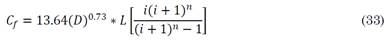
In order to calculate the fixed costs of the chosen pipes considering the various pipe sizes available in retail shops, the empirical mathematical formulation of the diameter-cost relationship was developed based on [1]. Fixed cost is determined using (33).
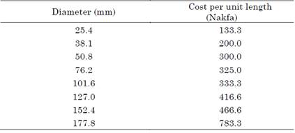
Additionally, the operating costs were calculated using (6). Based on the estimated fixed and operating costs of the different diameters available in the market and retail shops, the minimum value was selected for the various links, thus yielding the optimal economic diameter. Table 1 provides a detailed analysis of the optimal economic pipe size estimation for this case study using the mathematical equations included in the standard recommended LCCA model. In addition, it lists the different pipe sizes available in the retail shops.
Table 1 Available pipe diameters and their corresponding prices in the retail shops
Source: created by the authors.
The exponential-based empirical equation, given by (22), was deduced based on the information in Table 1. Figure 7 illustrates the relationship between pipe diameter and cost per unit length.
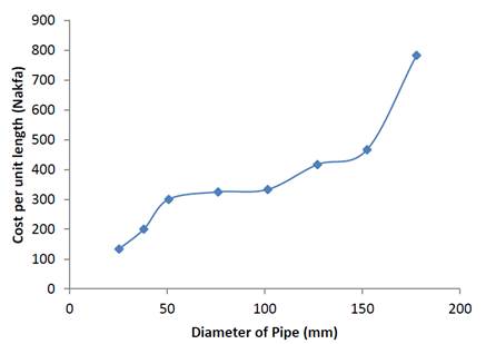
Source: created by the authors.
Figure 7 Relationship between pipe diameter and cost per unit length
Table 2 shows a detailed analysis of the optimal pipe size estimation for the case study using the mathematical equation proposed in [1].
Table 2 Optimal pipe diameter estimation using the standard life-cycle cost analysis model
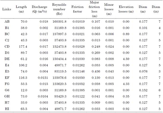
Source: created by the authors.
The network was assumed to be completely designed using PVC due to the benefits of this material. The pipes were considered to have a relative roughness of 1.5*10-6. The Reynolds number was determined using (34).
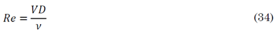
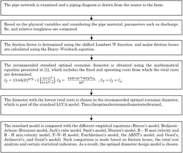
In this equation, Re denotes the Reynolds number; v, the average velocity in m/s; D, the diameter in m; and v, the kinematic viscosity in stoke. The friction factor was calculated using the Lambert’s W function based on (3), and the major friction losses were determined using the Darcy-Weisbach equation based on (1). The minor losses were assumed to be 10 % of the estimated major losses. A theodolite and a GPS were employed to measure the elevation of the agricultural plot. Once these values were estimated, the optimal pipe diameters were calculated using the mathematical equation included in the standard LCCA model. The diameter with the lowest fixed and operating costs based on the function of the different variables during the flow was considered to be the optimal pipe size for each link in the network. Figure 8 presents a schematic process flow diagram of the methodology implemented to compare and validate the optimal economic pipe diameter recommended for the case study.
3.2 Comparison of the estimated pipe diameters based on total friction losses
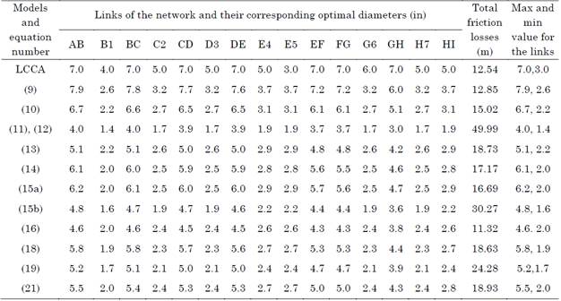
Table 3 provides a comparison of the various pipe diameters selected for the network at the HAC farm in terms of total head losses. Table 3 shows the total estimated friction losses during the flow, including major, minor, and elevation losses. The total losses calculated using the LCCA model were 12.54 m. The highest friction losses (49.99 m) were obtained using Jack’s Cube model (11 and 12), whereas the lowest friction losses (11.32 m) were yielded by the F-W-Hmodel (16). The diameter estimated using Jack’s Cube model was the smallest (1.4 in) of all the other diameters obtained with the eleven explicit empirical models. The largest diameter (7.9 in) was calculated by Bresse’s model (9). Moreover, Bresse’s model yielded a total friction loss, which was estimated to be closer to the standard LCCA model, of 12.85 m-slightly higher than that of the LCCA model (12.54 m). Another total friction loss value close to that of the LCCA model was the one provided by the model proposed by Bedjaouietet al. (10), with a value of 15.02 m. Forchheimer’s model (18), Smit’s model (13), and the model presented by Genić et al. (21) produced a very similar friction loss (ranging from 18.6 m to 18.9 m).
Table 3 Comparison of the optimal pipe diameters obtained using the different empirical models in terms of total head losses
Source: created by the authors.
The friction loss obtained with the B-H min.velocity model (15a) and Munier’s model (14) was higher than that of the model proposed by Bedjaoui et al. but lower than that provided by the other models. Finally, along with Jack’s Cube model, the ABNT’s model (19) and the B-H max.velocity model (15b) yielded one of the highest friction losses.
3.3 Comparison of the estimated pipe diameters based on the total cost analysis
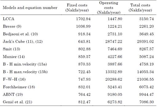
Table 4 provides a comparison of the selected optimal pipe sizes based on the total cost analysis. Both the fixed and operating costs of the selected pipes available in the retail market contribute to the total costs of the pipes in the network. The fixed costs of the various chosen diameters, which were determined using (4), depend on the interest rate and the lifespan of the pipes. The cost per unit length in (4) is estimated using the exponential form of the empirical equation given by (22). The operating costs of the pipes, which were calculated using (6), depend on the amount of water discharged into network, the friction factor, the cost of electricity, and the number of hours the pump is used to discharge water. Total costs which are computed using the mathematical equation in [1] and given by (7), is the sum of the fixed and operating costs.
Table 4 Comparison of the optimal pipe diameters obtained using the various empirical models based on total cost analysis
Source: created by the authors.
The total costs of the pipes chosen for the network, which were calculated using the standard mathematical equation [7] that is part of the recommended standard LCCA model, were 3150.74 Nakfa/year. The model proposed by Bedjaoui et al. (10) was found to yield a total cost close to that of the standard model, with a value of around 3649.45 Nakfa/year.
The total costs obtained with Bresse’s model (9) were 2261.20 Nakfa/year-lower than those of the LCCA model. The highest total costs were provided by Jack’s Cube model (11 and 12) and the F-W-H model (16), with a value of 29,391.02 and 21,036.55 Nakfa/year, respectively. The B - H min.velocity model (15a) and Munier’s model (14) yielded a total cost that was slightly higher than that of the model proposed by Bedjaoui et al. The total costs estimated by Forchheimer’s model (18), the model presented by Genićetal. (21), and Smit’s model (13) were higher than those of the standard LCCA model but lower than those of the ABNT’s model. Along with the F-W-Hmodel, the ABNT’s model (19) and the B-H max. velocity (15b) model produced one of the highest total costs.
3.4 Comparison of the empirical models with the standard LCCA model using various statistical indicators
The mathematical equation proposed in [1], which is the basis for the recommended standard LCCA model, was selected here as the benchmark and compared with the various empirical model equations, as it is widely accepted and used under a variety of reference conditions. Certain statistical indicators were employed to analyze the performance of the empirical equations in estimating the optimal pipe diameter for the network with the standard model.
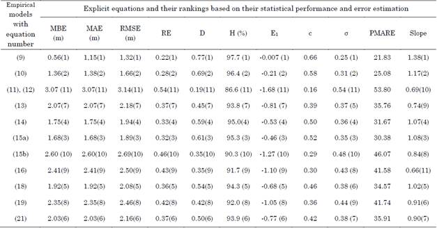
Based on some performance indicators and error criterion techniques, Table 5 compares the eleven explicit equations with the standard mathematical equation, given by (7), that is part of the LCCA model and ranks them accordingly. The value in brackets corresponds to each model’s ranking when compared to the others for each statistical parameter.
Table 5 Models’ comparison and ranking based on certain statistical performance indicators and error criterion estimation techniques
Source: created by the authors.
According to the Camargo and Sentelhas’ coefficient (‘c’), Bresse’s model had a “Regular” performance because its c value was 0.66. The model proposed by Bedjaouiet al. (10) and the B-H min.velocity model (15a) exhibited an “unsatisfactory” performance, as their c value was 0.55 and 0.52, respectively. Munier’s model (14), Forchheimer’s model (18), and the model presented by Genićet al. (21) showed a “bad” performance because their c value ranged between 0.41 and 0.50. The rest of the models had an “awful” performance, as their c value was lower than 0.40 for this case study.
The performance of the different models was ranked based on the PMARE between the observed and estimated values obtained with the standard and empirical equations. Of all the empirical models, the performance of Bresse’s model (9) and the model proposed by Bedjaouiet et al. (10) was classified as “moderate” because their PMARE value ranged between 20 % and 25 % and that of the other models as “unsatisfactory” because their PMARE value was higher than 25 %.
Based on the statistical indicators, i.e., MAE and RMSE, the performance of Bresse’s model (9) was almost accurate when compared to the standard diameter obtained using the mathematical equation of the LCCA model. The model proposed by Bedjaouiet al. (10) ranked second and was followed by the B - H min.velocity model (15a). Similarly, Jack’s Cube model (11 and 12), the B - H max.velocity model (15b), and the F-W-Hmodel (16) yielded higher value when compared to the standard LCCA model in this particular case study. Munier’s model (14), Forchheimer’s model (18), the model presented by Genićet al. (21), and Smit’s model (13) ranked almost better when compared to the standard model.
In comparison to the standard model, the RE obtained by Bresse’s model (9), the model proposed by Bedjaoui et al. (10), and the B - H min.velocity model (15a) was 0.22, 0.28, and 0.32 respectively. The MBE of Bresse’s model (9) ranked first, with a value of 0.56 m; that obtained by the model presented by Bedjaoui et al. (10) ranked second, with a value of 1.36 m; and that of the B-H min.velocity model (15a) ranked third, with a value of 1.68 m. As in the case of the MBE, the correlation ratio of Bresse’s model (9) ranked first, with a value of 97.7 %, followed by that of the other two methods, which ranked second and third, with a value of 96.4 % and 95.3 %, respectively. Jack’s Cube model (11 and 12) had the lowest correlation ratio (86.6 %).
When comparing the eleven empirical equations in terms of Willmott’s index, Legate and McCabe’s index, and standard deviation, Jack’s Cube model (11 and 12), the B - H max. velocity model (15b), the F-W-H (16), and the ABNT’s model (19) almost yielded higher values when compared to the standard LCCA model in this particular case study. After the three almost accurate models in this case study, Munier’s model (14), Forchheimer’s model (18), the model proposed by S.B. Genić et al. (21), and Smit’s model (13) had a good performance. In conclusion, Bresse’s model is the most adequate model to design optimal pipe sizes for the case study considered here. The model presented by Bedjaouiet et al. (10) and the B - H minimum velocity model (15a) can also be used to design optimal pipes following the previously mentioned method.
4. CONCLUSIONS AND FUTURE SCOPE
In the case study considered here, the goal was to design an optimal pipe size for the network at the HAC farm using the mathematical model proposed by Sonowal et al., which is part of the standard recommended LCCA model, as well as eleven other empirical equation models. The standard LCCA model was chosen to design the pipes because it is the standard method employed for any network. Despite this, it is often complex and requires large computations and a number of parameters to determine optimal pipe sizes. Therefore, a series of empirical equations that have been proposed by various authors can be employed to simplify the aforementioned procedure.
In comparison to the standard model, three models (Bresse’s model, the model proposed by Bedjaoui et al., and the B - H min. velocity model) performed fairly better. Although these three models performed better, some assumptions were considered when determining the total friction and total operating costs of the estimated pipe sizes. In the case of Bresse’s model, the value of coefficient k was assumed to be 1.50, and various studies have been conducted to enhance this model’s performance by properly choosing the value of k depending on the application. As suggested in [27], [38], k can take values ranging from 0.6 to 1.5. The model proposed by Bedjaoui et al. also takes into consideration various assumptions on which it holds: the installed capacity is directly proportional to the cost of the pumping station, and the pressure drop assumes a velocity of 0.8 m/s. The third model assumes a velocity of 3 ft/s, whereas the velocity is rarely kept constant in a nonlinear complex network.
Furthermore, Jack’s Cube model, the B - H max.velocity model, the F-W-Hmodel, and the ABNT’s model, which exceeded the ranking criteria in this particular case study, can be adjusted to perform better in certain cases. The F-W-H model, for instance, requires the head loss gradient to be determined, which was assumed here to be 2 m / 100 m, although the optimal pipe diameter value would vary accordingly depending on the estimated actual head loss gradient values. The remaining models (Smit’s model, Munier’s model, the model presented by Genić et al., and Forchheimer’s model) were found to perform relatively better than the aforementioned four models. Certain modifications and assumptions in the physical variables may lead to a better performance with respect to the most accurate performing models in this particular case study.
The design of optimal pipe sizes for the network at the HAC farm can be further expanded by means of more simplified empirical equations, which can be appropriately employed to design the pipeline network. In comparison to the mathematical equation of the recommended LCCA model, the value of coefficient k can be further improved using artificial intelligence optimization algorithms in order to obtain an accurate value for enhancing the resulting optimal pipe size.

