


 Inglés (pdf)
 Articulo en XML
 Referencias del artículo
 Enviar articulo por email
 Citado por SciELO
  Citado por Google
  Similares en
SciELO
Similares en
SciELO  Similares en Google
 Permalink
1. INTRODUCTION
Population growth, technology advances, infrastructure, and greenhouse gases have caused the electric energy demand to increase disproportionately in the last years around the world [1]. An example of this is the increased use of electric vehicles (EVs), which have required an accelerated strengthening of the electric systems infrastructure with the objective of meeting the electric energy demand while also considering a sustainable future thanks to the low CO 2 emissions of EVs. This type of vehicles contributes to mitigating air pollution problems, which makes them attractive for consumers [2]. All of this is linked to the multiple mechanisms and proposals that have been made for governmental entities to reach common objectives like Net-Zero 2050, which consists of preventing an increase in the earth’s average temperature 1.5 °C over the current values, thus achieving 0 % CO 2 emissions by 2050 [3].
The electric energy demand in 2020 was 23300 TWh. By 2030, 30000 TWh are expected[4]. To meet that demand, it is necessary to broaden the use of electric energy, and, considering the objectives mentioned above, it is necessary to incorporate technologies with renewable sources as their primary energy input. The energy supply growth through renewable energy sources has been increasingly promoted. For example, the wind and solar power generated in 2020 was 93 GW and 139 GW, respectively [5], [6].
Increasing the renewable energy capacity brings a number of challenges. Among these are the mechanisms for integration to the electricity market and their effects on the price of electricity [7], as well as the impact and participation of power systems modeling and optimization in the search of intelligent network development [8]. On the other hand, power systems control is an important challenge to overcome regarding optimal systems operation. Furthermore, converter control is also among these challenges with respect to their integration to power systems (such as VSCs, FACTs, etc.), due the fact that their operation depends on the energy source and the power system itself. Thus, converters could connect to energy networks and improve their behavior [9]. In this context there are different kind of controls which have been implemented in both converters and inverters. Particularly, the direct current converter control involves a diversity of techniques [10] - [12], namely, direct pole placement [13]; voltage control mode [14]; current control mode [15], [16]; PID control[17]; classical half cycle posicast control [18]; hybrid posicast control [19]; sliding control mode [20]; fuzzy logic control [21], [22]; neural network-based control [23]; predictive model control [24]; state space modeling control and passivity-based control [25], [26]; and intelligent control, among others. These techniques allow achieving and/or satisfying the demands of problems in specific systems. An example of this is improving the behavior of the converters’ dynamic response, increasing the efficiency, and reducing their own power losses. To summarize the main literature reports in the current literature regarding control and its applications in DC-DC converters, Table 1 lists important reference works that have dealt with control designs in the converters under study.
Table 1 Background of some control techniques used in DC-DC converters
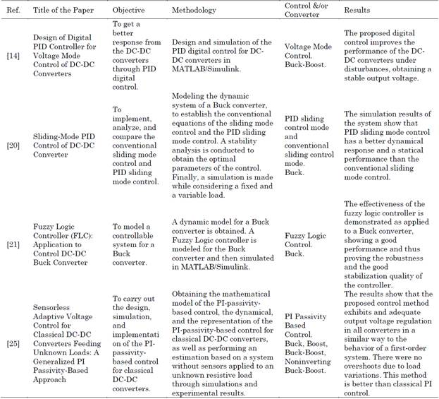
Source: created by the authors.
It is important to mention that, despite having been generally addressed in the scientific literature for DC-DC power converters [27] - [29], inverse optimal control has not been addressed as it is in this document. The papers [27] - [29], only describe the inverse optimal control for the Boost converter. For that reason, the following contributions from this research are presented:
-A general methodology to implement inverse optimal control theory to any second-order DC-DC converter for voltage regulation in generic resistive loads.
The addition of integral gain to the classical inverse optimal control design in order to reduce possible steady state errors in the voltage regulation caused by unmodeled dynamics in DC-DC converters.
The explicit demonstration of the stability in closed-loop operation for all the DC-DC converters studied via Laypunov’s stability theory.
The structure of this paper is as follows: Section 2 summarizes the main definitions and aspects that contribute directly to the research; Section 3 presents the general modeling for studied classical second-order DC-DC converters; Section 4 presents dynamic modeling as a function of the error of the state variables for the studied second-order DC-DC converters; Section 5 presents the implementation of inverse optimal control while adding proportional and integral action for the studied classical second-order DC-DC converters; Section 6 presents the numerical validation and analysis of the implemented inverse optimal control for the studied converters through simulations of the voltage and current dynamic response via the PSIM software, which is in turn compared with open-loop control and other types of nonlinear control (PI passivity-based control), using the parameters described in [26]; and finally, Section 7 presents the conclusions and future work.
2. METHODOLOGY
2.1 Reference framework
2.1.1 State space modeling
State space modeling is a way to represent the dynamic equations of a system, which consist of a set of first-order differential equations where the variables are known as state variables. This kind of equations are particularly useful in modern control theory [30], [31]. These equations are a canonical form to write the differential equations that describe the dynamical behavior of a system. In the case of converters, state variables are associated with the elements that store energy, i.e., capacitors and inductors. In the case of capacitors, the state variable is the voltage and in the inductors are the current [30]. State variables must satisfy these two conditions [31]:
At any initial time t=t 0 , state variables define the initial state of the system.
Once the input of the system for t ≥ t 0 and the initial states defined above are specified, the state variables must completely define the behavior of the system in the future.
Therefore, state variables “are defined as a minimum set of variables x 1 (t), x 2 (t), ..., x n (t), whose knowledge in any time t 0 , and the knowledge of the excitation input information that is applied subsequently, are enough to find the state of the system at any time t > t 0 ” [31]. The state equations can be represented in the form of a matrix, as is shown in (1) [30], [31]:
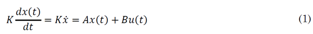
Where x(t) is the vector that contains the state variables; u(t) is the input vector that contains the independent inputs to the system (as an example, it could be the voltage of the input source in a converter); x ̇ is the derivative of the state variables vector; K is the vector that contains the respective elements (in the case of the converters, it would be the capacitances, inductances, and mutual inductances, if any); and the A and B matrices contain proportionality constants.
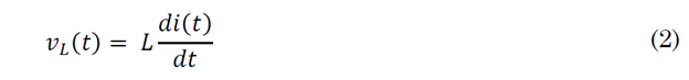
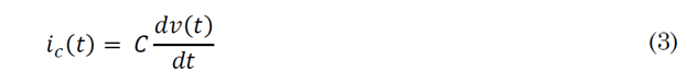
As state variables are the voltage (in volts - V) and current (in amperes - A) of the capacitor and the inductor, respectively, as shown in (2) and (3), it is necessary to define what these two variables are:
If we refer to second-order converters, it is necessary to consider both state variables, thus making it possible to find the state equations. Thereupon, it is important to consider the two states of the switch in the converter. The two states are added, knowing that A 1 and B 1 refer to when the switch is on and A 2 and B 2 to when the switch is off. Then, (4) is obtained[30], [32]:

Where D ϵ [0-1] is the control variable (also known as u) and D' = 1-D. This variable is dimensionless.
2.1.2 Inverse optimal control
The optimal control of a system implies finding the best approximation of an objective depending on a given performance criteria [33]. This control seeks to find all the performance indices for which a given control law is optimal [34]. In addition, this avoids the explicit solution of the Hamilton-Jacobi-Bellman equation (HJB), which establishes the beginning of optimal control, in order to find the optimal control law [35]. Optimization, i.e., either maximizing or minimizing (depending on the system requirements), is carried out through a cost function or performance index associated with system variables such as the error, the control signal, and the state vector. This function has the form shown in (5) [27], [28], [34] - [36]:

Where J(x(t),u(t)) is the cost function (also known as performance index) that represents the cumulative contribution over time; L\{x(t),u(t)\} is known as the loss or Lagrangian function, which is the soft function that depends on t, x, and u, (it is also a continuously differentiable function with respect to x(t) and u(t)); l(t)≥0 represent the weighing error; x(t) is the state vector ϵ R n ; u(t) ϵ R m is the control vector; R(x)>0 ∀ x(t); and T denotes the transpose of the matrix.
In the inverse approximation, the stabilizer feedback is first designed, and then it is demonstrated that is optimal for the cost function J(x(t),u(t)). It is said that the problem is inverse because the functions l(x) and R(x) are determined by the stabilizer feedback instead of being chosen a priori by the designer [36]. The stabilized control law u(x) answers the optimal inverse control problem for the system with (6) [27], [28], [34]-[36]:

Where f: R n →R n and g: R n →Rnxm are generally nonlinear functions of the state. When Jis minimum, it is known as the function of optimal value, which is regarded as the Lyapunov function denoted by V(x). If u(t) is optimal, it is denoted as u*. To find the optimal control law, it is necessary to define the associated Hamiltonian of the system, which is given by (7) [27], [35]:

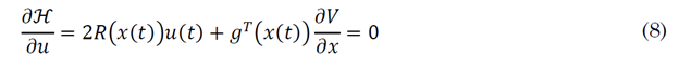
To ensure optimality,  = 0 is required, so (7) can be rewritten as is shown in (8):
Equation (9) is given after clearing (8):

The equation above is the optimal control law and can be written in a formal way using the following theorem [27], [35], [36]:
-Theorem 1 (sufficient condition for optimality): If a positive semidefinite function V(x) exists which is differentiable once C 1 , that satisfies the HJB, (10) is obtained:

where l(x) and R
-1
(x) are given by the cost function, while f(x) and g(x) by the system, then the control law shown in (9) ensures global asymptotic stabilization at the equilibrium point. Thus, u* (x) is the stabilizer inverse optimal control that minimizes the cost function, guaranteeing that  x(t)=0 and V(x) is the optimal value function. To solve the optimal control problem, it is necessary to solve (10).
2.1.3 Lyapunov theorem
A system is stable, according to Lyapunov, if the function V(x) satisfies the following set of conditions [37]:
Condition 1. ∀x = 0, the chosen Lyapunov function for his point must be equal to zero, as shown in (11).

Condition 2. ∀x ≠0, the chosen Lyapunov function must be greater than zero, as shown in (12).
Condition 3. The chosen Lyapunov function derivative with respect to time must be lower than zero, as shown in (13).

If the three conditions above are fulfilled, then the system is stable.
2.1.4 DC-DC converters
A DC-DC converter is a power electronic circuit that allows conversion between DC voltage levels by stepping up or down the voltage. These circuits can be controlled through different methods that involve regulating the voltage for it to remain constant when there are load variations.
In general, all converters consist of inductors, capacitors, diodes, and transistors. Inductors and capacitors act together as a low-pass filter to remove the harmonics produced by the transistor’s commutation in order to only allow the DC component to pass to the load [30]. To keep the input and output power equal, it is mandatory that the converters step up or down the current depending on the converter [26].
For DC-DC converters, an analogy can be made with a transformer, which works with AC signals while DC-DC converters work for DC signals for the sake of redundancy.
To control the converters, a PWM is needed (the most classical control). Two states of the transistor are given: on and off. The PWM interval is the duty-cycle that is the amount of time that the transistor is in on state or off state as a percentage of the total time of it takes to complete one cycle, and is between 1 and 0, and, depending on the converter topology, it helps to step up or down the output voltage.
2.2 Proposed methodology
Figure 1 shows the methodology used to model the converters and obtain the functions that describe the control laws for each of them.
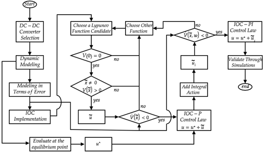
The first step is to choose the converter for which the control law will be obtained to later implement the dynamic modeling (state equations) of the chosen converter. The obtained state equations must be evaluated in the equilibrium point to get u*, and they must also be written in terms of error. Then, the inverse optimal control can be implemented, where the Lyapunov candidate function must be chosen first. This function must satisfy conditions 1 and 2 of the Lyapunov theorem, so u can be obtained. Condition 3 of the Lyapunov theorem can then be evaluated. If this condition is satisfied, then the inverse optimal control with proportional action law is obtained. Afterwards, an integral action is added, and condition 3 of the Lyapunov theorem is evaluated. If the condition is satisfied, then the inverse optimal control with proportional-integral action is obtained. Finally, numerical validation is made to evaluate the control law that was found through simulation.
2.3 General modeling of classical DC-DC converters
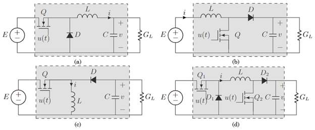
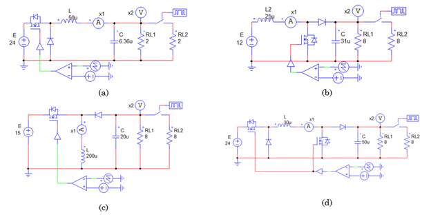
This section presents the general dynamic modeling of the most classical DC-DC converters. The studied topologies are Buck, Boost, Buck-Boost, and Noninverting Buck-Boost converters. The general characteristic of these kind of converters is that they are classified as second-order converters since each of them presents two associated dynamics (current and voltage of the inductor and capacitor, respectively). Figure 2 shows the studied converters’ general structure. These are connected to a resistive load, which is modeled as a conductance G L .
Source: created by the authors.
Figure 2 Second-order DC-DC converters: (a) Buck converter, (b) Boost converter, (c) Buck-Boost converter, (d) Noninverting Buck-Boost converter
Variables and parameters in Figure 2 have the following interpretation: E>0 corresponds to the input voltage (in volts - V); i>0 represents the associated current of inductor L (in amperes - A); v represents the output voltage associated to capacitor C (in volts - V); and u ϵ [0-1] represents the input control variable applied to the forced commutation of the transistors (dimensionless quantity) [25]. To obtain the state equations of the converters (Figure 2), it is necessary to use Kirchhoff’s current and voltage laws in the two states in which the converters operate (with Q on and Q off) [26]. Kirchhoff’s laws must be applied both in the mesh that contains the inductor and in the node in which the capacitor is located within each state. To obtain the dynamic model of the DC-DC converters, the following assumptions must be made [26]:
Assumption 1. The power losses, both in the transistor Q and the diode D, are neglected.
Assumption 2. The input voltage and the state variables (current and voltage of the inductor and capacitor respectively) are measurable.
Assumption 3. The converter parameters (inductor L and Capacitor C) are positive definite.
Assumption 4. The value of the constant resistive load (modeled as a conductance) is bounded and positive.
Assumption 5. The switching frequencies are sufficiently high to employ the average modeling theory.
By renaming the state variables and then deriving them, we have (14) [32]:
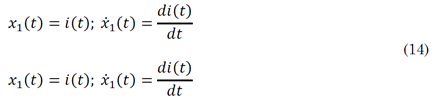
Equations above are the renamed equations of state variables. x 1 is the current in the inductors and x ̇ 1 its derivative; x 2 is the voltage in the capacitors and x ̇ 2 its derivative.
2.3.1 Buck converters
Buck converters (also known as step-downs or ‘Choppers’ - Figure 2a) are a type of DC-DC converter intended for stepping down the voltage [30]. Their most common application is to regulate the output voltage for load variations [26]. By using the Kirchhoff laws, (15) and (16) are obtained:


Equations above are the state equations that describe the dynamical behavior of the Buck converter.
2.3.2 Boost converters
DC-DC converters are also called step-ups (Figure 2b) because the output voltage is greater than the input voltage. Their main application is in the DC-regulated energy sources and DC motor regenerative speed braking [38]. By using the Kirchhoff laws, (17) and (18) are obtained:


Equations above are the state equations that describe the dynamical behavior of the Boost converter.
2.3.3 Buck-Boost converter
This type of converter (as shown in Figure 2c) is the cascade connection of Buck and Boost converters. The output voltage can be lower or greater than the input voltage, and it has an opposite polarity to the input voltage. By using the Kirchhoff laws, (19) and (20) are obtained:


Equations above are the state equations that describe the dynamical behavior of the Buck-Boost converter.
2.3.4 Noninverting Buck-Boost converter
This type of converter is similar to Buck-Boost converters. The difference is that the output voltage polarity has the same as the input voltage. These converters, compared to their homonymous, have two transistors and two diodes that are commuted at the same time in the corresponding interval (Q 1 and Q 2 in interval 1, and D 1 and D 2 in interval 2 -Figure 2d). Their voltage output also can be greater or lower than the input voltage. By using the Kirchhoff laws, (21) and (22) are obtained:


Equations above are the state equations that describe the dynamical behavior of the Noninverting Buck-Boost converter.
2.4 Dynamic modeling in function of the error
To obtain the error model of the converters, it is necessary to begin with their dynamic equations, namely (15) to (22). The analysis of the model must be evaluated at the equilibrium point x*, which is equivalent to zero (x* = 0) and then fx* = 0, as well as at the equilibrium point, u* = 0. The equations (23) and (24) following variables are needed:


Moreover, the dynamic error behavior must be considered. The equations (25) and (26) represent the error:


Where,  is a vector that represents the error and has the same dimension as the state variables vector that contains the error of current
  and the voltage of the capacitor
  and
and  is the input control variable (ideally, the error must be equal to zero). To obtain x*, the state equations must be evaluated at the equilibrium point. This is important because the system signals are constants, and the derivative at the equilibrium point is therefore zero. To demonstrate the procedure, modeling will be carried out with the Buck converter. However, the procedure is the same for all converters.
2.4.1 Buck converter modeling
For the current state equations, the model is not satisfied. This is because the function is not equal to zero. Evaluating at the equilibrium point, we have (27) and (28):


Clearing equations above, (29) and (30) are given:


Equations (29) and (30) is the control law u* ϵ [0-1] at the equilibrium point and (30) is the current x* 1 in terms of the output voltage x* 2 at the equilibrium point, show that we are working with a Buck converter. It is important to remember that the control law is given by the ratio of the output voltage over the input voltage for this converter [39] and that x 2 = v, as expressed by (14). The control can be implemented with the steady state variables and a basic PWM. However, the problem is that the desired response takes a long time to stabilize.
For the control law, u* was obtained. Now, the objective is to obtain . First, (25) and (26) are replaced in the dynamic equations of the converter obtaining (31) and (32):


Equations above demonstrate how the error is implemented in state equations and can be reduced using (27) and (28), as is shown in (33) and (34):
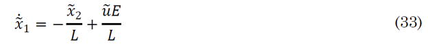
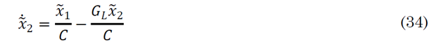
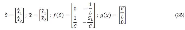
Equations above are the simplified equations in terms of the error and can be rewritten in matrix form as is shown in (35):
It’s important to mention that the equilibrium points of  =0. This is because x = x* is desirable.
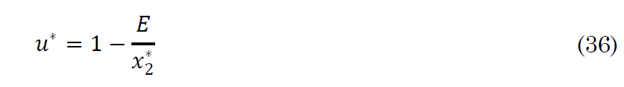
2.4.2 Boost converter modeling
Like the Buck converter, the error model for the Boost converter can be obtained using the dynamical equations. Equations (36) and (37) show that we are working with a Boost converter [39].

By adding the error to the system through (25) and (26) in (17) and (18) and simplifying, (38) and (39) are obtained:
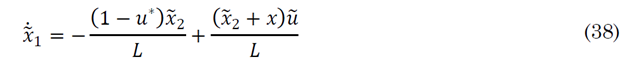

The equations above are the simplified equations in terms of the error and can be rewritten in the form of a matrix, as is shown in (40).

2.4.3 Buck-Boost converter modeling
Using the dynamic equations at the equilibrium point, (40) and (41) are obtained:
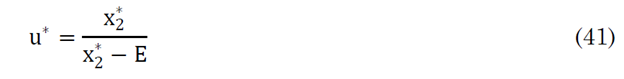

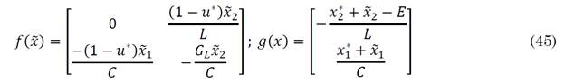
Equations (41) and (42) show that we are working with a Buck-Boost converter [39]. By adding the error to the system through (25) and (26) in (19) and (20) and simplifying, (43) and (44) are obtained:

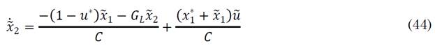
The equations (43) and (44) are the simplified equations in terms of the error and can be rewritten in the form of a matrix as is shown in (45).
2.4.4 Noninverting Buck-Boost Converter
Using the dynamic equations at the equilibrium point, (46) and (47) are obtained:

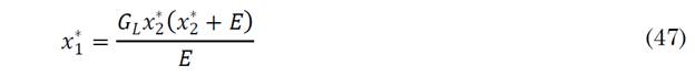
Equations (46) and (47) show that we are working with a Noninverting Buck-Boost converter [40]. Adding the error to the system through (25) and (26) in (21) and (22), and simplifying, (48) and (49) are given:


The equations (48) and (49) are the simplified equations in terms of the error and can be rewritten in the form of a matrix, as is shown in (50).

2.5 Inverse optimal control implementation
To implement inverse optimal control (IOC) in the converters, it is necessary to first choose a Lyapunov function. In this case, (51) is the candidate function:

Equation (47) is a function that satisfies conditions 1 and 2 of the Lyapunov theorem, as shown in (11) and (12). Condition 3 must be verified. If another function is selected, we can obtain another control law. To demonstrate the third condition, the IOC implementation to the Buck converter will be shown. However, the procedure is the same for all converters.
2.5.1 Buck converter
-Proportional control law: Regarding (9),  , and must be found. For the Buck converter, (52)-(54) are given:
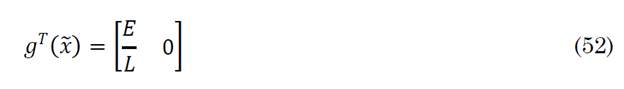
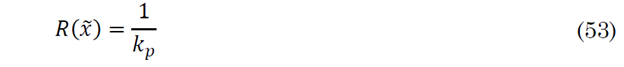

Equations (53) and (54) are a constant and the partial derivative of the Lyapunov candidate function respectively, necessary to find the optimal control law (9) for the buck converter and are the same for all converters. Replacing (52), (53), (54) in (9), (55) is obtained:
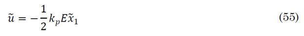
Equation (55) is the error in (26) and is obtained by the optimal control law theory. By replacing (29) and (55) in (26), the proportional control law (56) is obtained:

-Demonstration of condition 3 of the Lyapunov for the selected function regarding the proportional (P) control law: Equation (51) is derived in terms of time, obtaining (57):

Which is the derivative in terms of time of the Lyapunov function candidate. Equations (33) and (34) are replaced in (57), obtaining (58):
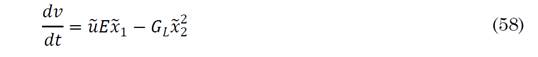
Equation (51) is replaced in (58), obtaining (59):
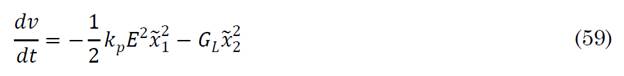
Equation (59) demonstrates the third condition and is also satisfied as long as . This allows us to conclude that the proportional control law is asymptotically stable because the control variable depends on both state variables. In case one of the state variables disappeared from the control variable, the control law would be only stable.
-Proportional-Integral (PI) control law: In this case, an integral action must be added, as is shown in (60) and (61):

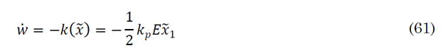
In (60) and (61) is shown how is implemented the integral action in the optimal control law (9) for the buck converter. Considering (29) and (60), (62) is obtained:

The control law shown in (62) must be simplified by replacing , then we have the Proportional-Integral control law (63):

Equation (63) shows an optimal Proportional-Integral controller because the procedure comes from the IOC theory. This control scheme generates a PI control that guarantees stability all over the system, which is also optimal. It is important to mention that, in the controller, despite the control action given by current, the voltage is controlled. This can be observed in (30).
-Demonstration of condition 3 of the Lyapunov theorem for the selected function regarding the PI control law: By adding the integral action, the Lyapunov function yields (64):

Equation (64) is the Lyapunov candidate function for the PI control law for the Buck converter. Deriving in terms of time, (65) is obtained:

Equations (33), (34), and (61) are replaced in (65), which is the derivative of the Lyapunov function candidate (66):

The control law shown in (66) must be simplified by replacing , obtaining (67):

Equation (67) is the same as (59). However, in this case, the control is stable because the variable w disappears.
2.5.2 Boost converter
-P control law: The P control law for the Boost converter is shown in (68):

Equation (68) is obtained by replacing (36) and the respective error for the Boost converter.
-Demonstration of condition 3 of the Lyapunov theorem for the selected function regarding the P control law: The equation that demonstrates the third condition of the Lyapunov theorem is shown in (69):

Equation (69) is obtained by deriving de Lyapunov candidate function for the Boost converter.
-PI control law: Equation (70) is the PI control law:

Equation (70) is obtained by replacing (36) and the respective error with PI action for the Boost converter.
-Demonstration of condition 3 of the Lyapunov theorem for the selected function regarding the PI control law: Equation (71) demonstrates the third condition of the chosen Lyapunov function:
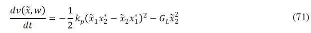
Equation (71) is the same as (69). However, in this case, the control is stable because the variable w disappears.
2.5.3 Buck-Boost converter
-P control law: The P control law for the Buck-Boost converter is shown in (72):

Equation (72) is obtained by replacing (41) and the respective error for the Buck-Boost converter.
-Demonstration of condition 3 of the Lyapunov theorem for the selected function regarding the P control law: Equation (73) demonstrates the third condition of the Lyapunov theorem:

Equation (73) is obtained by deriving de Lyapunov candidate function for the Buck-Boost converter.
-PI control law: Equation (74) is the PI control law:

Equation (74) is obtained by replacing (41) and the respective error with PI action for the Buck-Boost converter.
-Demonstration of condition 3 of the Lyapunov theorem for the selected function regarding the PI control law: Equation (75) demonstrates the third condition of the chosen Lyapunov function is the following:

Equation (75) is the same as (73). However, in this case, the control is stable because the variable w disappears.
2.5.4 Noninverting Buck-Boost converter
-P control law: The P control law for the Noninverting Buck-Boost converter is shown in (76):

Equation (76) is obtained by replacing (46) and the respective error for the Noninverting Buck-Boost converter.
-Demonstration of condition 3 of the Lyapunov theorem for the selected function regarding the P control law:
Equation (77) demonstrates the third condition of the chosen Lyapunov function:

Equation (77) is obtained by deriving de Lyapunov candidate function for the Noninverting Buck-Boost converter.
-PI control law: Equation (78) is the PI control law:

Equation (78) is obtained by replacing (46) and the respective error with PI action for the Noninverting Buck-Boost converter.
-Demonstration of condition 3 of the Lyapunov theorem for the selected function regarding the PI control law: The equation (79) demonstrates the third condition of the chosen Lyapunov function:

Equation (79) is the same as (77). However, in this case, the control is stable because the variable 𝑤 disappears.
3. RESULTS AND DISCUSSION
The controls where numerically validated via simulations with the PSIM software, version 2021a, where open-loop control and closed loop control simulations were performed. The objective of these simulations was to show the dynamic response of the converters. For the closed loop control, the inverse optimal control with PI action (IOC-PI) and the PI passivity-based control (PI-PBC) were implemented in order to compare two kinds of nonlinear control [25], [26]. The study was conducted with the values proposed by [26] with a switching frequency of 100 kHz. Table 2 presents these values.

3.1 Numerical validation
As well as [26], the following validations were considered to demonstrate the effectiveness of and strengthen the proposed IOC-PI controller in order to regulate the output voltage of the second-order DC-DC converters:
The initial voltage of the capacitor was equal to the reference voltage x* 2 , also called v (Table 2). The current in the inductors, due to convergence problems in the simulator, was considered to be 0 A.
The system was initially positioned with the load G L2 . In the simulator, there were two loads with the same value G L1 in parallel. After 2.5 ms, the load changed, leaving a single load equal to G L1 . This process was repeated twice for a total time of 10 ms.
All simulations were validated in an interval of 10 ms.
It is important to mention that all simulations were run after the state variables stabilized in the simulator. In this case, the simulations shown took between 0.09 seconds and 0.1 seconds, enough time to see the dynamic response considering the load variations. The settling time (t s ) and the steady-state error (ε ss ) were used to quantify the performance of both the nonlinear controller (IOC-PI and PBC-PI) and the open-loop control.
3.2 Open-loop control
Figure 3 shows the implemented circuits with open-loop control in the software. Figure 3a, Figure 3b, Figure 3c and Figure 3d are the open-loop control for the Buck, Boost, Buck-Boost and Noninverted Buck-Boost converter respectively implemented in PSIM. In this case, only a comparator was used where the inputs were a sawtooth signal with a maximum voltage of 1 V and a 100 kHz frequency, as well as a reference signal corresponding to the duty cycle u (Table 2).
Source: created by the authors.
Figure 3 Open-loop control of the implementation of second-order DC-DC converters in PSIM: (a) Buck converter, (b) Boost converter, (c) Buck-Boost converter, (d) Noninverting Buck-Boost converter
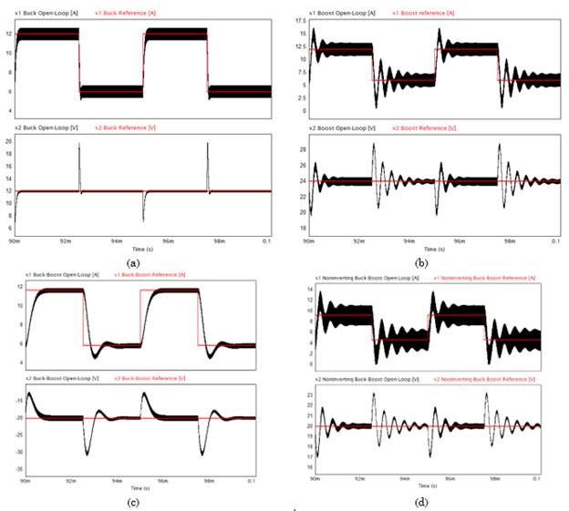
Figure 4 shows the dynamic response of the output voltage and the current of the inductors of the converters in open-loop control. Figure 4a, Figure 4b, Figure 4c and Figure 4d are the open-loop control dynamic response for the Buck, Boost, Buck-Boost and Noninverted Buck-Boost converter respectively. All the open-loop simulations are described as follows: x 1 (inductor current) and x 2 (output voltage), in black, are the output current voltage respectively; x* 1 and x* 2 , in red, are the reference inductor current and reference output voltage. The load variations are remarkable: each 2.5 ms in all converters. Boost, Buck-Boost, and Noninverting Buck-Boost converters have a slow dynamic response compared to the buck converter. This is due to the nonlinearity of these converters (the Buck converter is linear).
3.3 Closed-Loop control
For the PI-PBC controller, the gains K p and K i were chosen in accordance with [26] (see Table 3). For the IOC-PI controller, the gains K p and K i in each converter were tuned to 0.5 and 0.1, respectively (these control gains were found by implementing a heuristic search algorithm that minimizes the mean square error between the voltage reference and the converters’ output). All the closed-loop simulations can be described as follows: in each figure, the voltage and current dynamic responses of the IOC-PI and PI-PBC controllers are compared; the inductor current (x 1 ) is the upper graph, and the output voltage (x 2 ) is the lower graph; the PI-PBC validation is presented in black and the IOC-PI validation in red.

3.3.1 Buck converter
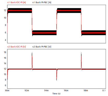
Figure 5 shows the dynamic response of both nonlinear controllers for the Buck converter. In the IOC-PI controller, the peaks and valleys in the voltage signal, ripple, and settling time are lower than those in the open-loop and PI-PBC controllers. The peaks in the voltage signal go from 19.74 V in open-loop control to 17.94 V in the PI-PBC controller, and finally to 16.77 V in the IOC-PI controller. The valleys in the voltage signal go from 7.03 V in open-loop control to 7.82 V in the PI-PBC controller, and finally to 8.58 V in the IOC-PI controller. The IOC-PI controller shows a better performance in all parameters when compared to the open-loop and PI-PBC controllers. It should be highlighted that both nonlinear controllers manage to achieve a reduction of the settling time and ripple with respect to the open-loop control (Figure 4a). Both controllers keep the voltage around the reference voltage despite the load variations. The steady state error is better in the open-loop control, but the settling time is better in the IOC-PI controller (Table 4).
Source: created by the authors.
Figure 5 Dynamic response of the output voltage and inductor current of the IOC-PI (red) and PI-PBC (black) controllers of the Buck converter in PSIM

3.3.2 Boost converter
Figure 6 shows the dynamic response of both controllers (PI-PBC and IOC-PI) for this converter. Both controllers clearly have a better response compared to the open-loop control (Figure 4b), but the IOC-PI controller has the best response among the three controllers with regard to the steady state error (Table 4) and the ripple.
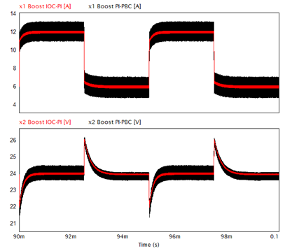
Source: created by the authors.
Figure 6 Dynamic response of the inductor current and output voltage of the IOC-PI (red) and PI-PBC (black) controllers of the Boost converter in PSIM
The controllers have a similar response, as well as have peaks and valleys of 26 V and 21.5 V, respectively, but the voltage is maintained at the reference despite the load variations. The settling times in both cases are very similar; thus, it is assumed that this happens at the same time. The ripple in the IOC-PI controller has a considerable reduction regarding the open-loop and PI-PBC controllers.
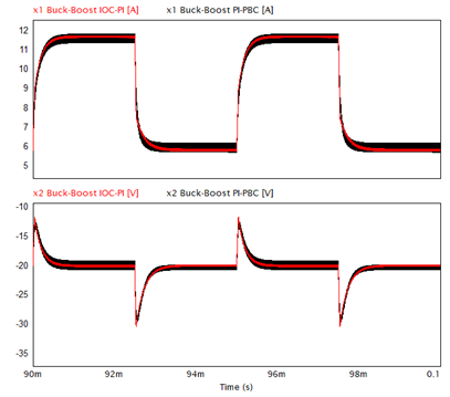
3.3.3 Buck-Boost converter
The dynamic response of the Buck-Boost converter is shown in Figure 7. Like the dynamic responses of the converters above, the controllers have a better response than the open-loop control (Figure 4c), and the output voltage is within the reference values. In both cases, although the dynamic response is very similar, there is a significant reduction of the ripple in the IOC-PI controller regarding the PI-PBC controller, and, although the controllers have peaks and valleys in the voltage signal around -12.5 V and -30 V, they are lower than those of the open-loop control. In this case, the settling time is assumed to be the same (see Table 4) in both implemented nonlinear controllers. The steady state error is lower in the IOC-PI controller (see Table 4).
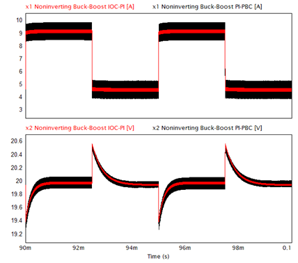
3.3.4 Noninverting Buck-Boost converter
Figure 8 shows the dynamic response for the implemented nonlinear controllers of this converter. The dynamic response in both controllers is better than the open-loop control, where, despite the load variations, the output voltage is at the reference. The peaks and valleys for the controllers decrease in comparison with the open-loop control (Figure 4d). The settling time is assumed to be the same for both controllers, and it is better than the open-loop control. The PI-PBC controller has a lower steady state error than the IOC-PI controller and the open-loop control (see Table 4). It is important to highlight that the ripple shows a significant reduction in the IOC-PI controller.
4. CONCLUSIONS AND FUTURE WORK
Dynamic models of classical second-order DC-DC converters in terms of the error were obtained, which allowed determining the control law through inverse optimal control theory. A closed-loop controller was designed which allowed observing the dynamic response of different converters, thus concluding that the system was stable according to the Lyapunov theorem. The PI-PBC control law designed in [26] was compared with the IOC-PI control law implemented in this document. The numerical results showed that both control laws are dynamically better than open-loop control, and that the IOC-PI controller is the one with the best response.
Furthermore, it is necessary to clarify that all the converters have a fairly pronounced ripple, and, despite the fact that the gains helped reduce it, it can be improved. Therefore, in order to reduce it both in the output voltage and in the current of the inductors, a detailed design of the converters must be carried out, choosing the capacitors and inductors according to the required design parameters.
To compare the two implemented control laws, Figure 9 shows the implementation of a Boost converter with both controllers. The number of elements used in the IOC-PI controller is far less than in the PI-PBC controller, which leads to a simpler implementation, reduced simulation/execution times, and a reduction of human errors while implementing the control law, among others. This makes the control law proposed in this document optimal, since it uses fewer resources to reach the same or a better solution. In addition, it is noteworthy that the simulation time in the IOC-PI control law was far less than in the PI-PBC control law.
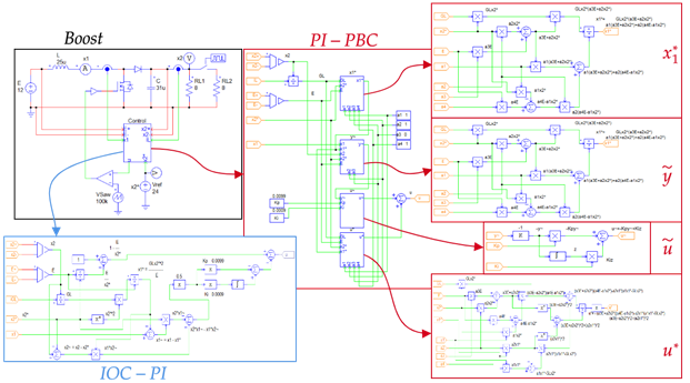
Source: made by the authors.
Figure 9 Block diagrams implemented for the Boost converter in PSIM. The converter is presented in black, the IOC-PI controller in blue, and the PI-PBC controller in red
The implementation of the inverse optimal control is proposed as future work, considering the switching losses of the transistor, the internal resistance and forward voltage of the diodes, and the internal resistance of the elements that store energy. Furthermore, implementation in fourth-order converters could be carried out, such as the Ćuk, SEPIC, and Zeta converters, as well as the implementation in DC/AC systems involving VSCs and AC/AC systems such as inverters.

