


 Inglés (pdf)
 Articulo en XML
 Referencias del artículo
 Enviar articulo por email
 Citado por SciELO
  Citado por Google
  Similares en
SciELO
Similares en
SciELO  Similares en Google
 Permalink
1. INTRODUCTION
A pavement transition is used to connect two pavement types and/or sections in order to provide a smooth and gradual change in the structural capacity of the pavement [1], [2]. Three methods have been reported in the literature to adequately construct an ACP-PCCP transition. One method consists of constructing a CS with variable thickness (transition slab) between the ACP and PCCP, which allows for gradual change of thickness and deflections; however, this technique is applied when there is sufficient distance between the pavements[3]. The other two methods are used when there is a sudden change from ACP to PCCP. One technique consists of cutting a 1 ½-inch wide joint at the AC-concrete interface comprising the entire thickness of the AC to be filled with elastomeric concrete, and the other consists of removing AC and concrete in the vicinity of the joint in order to compact a patching mix composed of gravel and fiber-reinforced polymer patching binder [1].
On the other hand, the literature states that distresses in ACP-PCCP transitions are mainly experienced near the joint. The distresses reported consist of the opening of the joint that may cause water to enter the pavement; settlement of the CS; distortion, material heaving, and bumps in the AC [1]-[3]. In addition, it is reported that distresses may be caused by 1) differential deflection between AC and CS due to the difference in stiffness between both materials; 2) excessive deflection of the CS edge that could affect the subgrade, and 3) poor quality of transition construction [2]-[4].
1.1 Background
In Bogotá, Colombia, extensive stretches of PCCP were built exclusively for bus rapid transit (BRT) that integrates the TransMilenio transportation system. Due to various factors, some CSs have experienced distresses and the repair of the PCCP consisted of replacing the CSs with continuous dense gradation AC with 19 mm nominal maximum aggregate size (NMAS). Therefore, during the repairs, sections of the PCCP were converted to ACP, i.e., ACP-PCCP transitions were constructed.
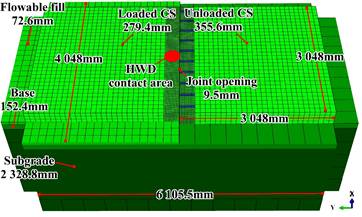
It is worth mentioning that the ACP-PCCP transitions were not constructed with methods such as transition slab, elastomeric concrete joint, or patching mix, instead, the pavement transitions consisted solely of the sudden change from AC to CS (direct ACP-PCCP transitions). Nevertheless, prematurely in some direct ACP-PCCP transitions, the AC began to experience cracking and material heaving, mainly under the tire path and near the joint, as well as differential displacement of the joints (Figure 1). Currently, the origin of the distresses has not been investigated and remains uncertain. Although the literature reports possible causes of distresses for ACP-PCCP transitions, these do not allow an understanding of the failure mechanisms of a direct ACP-PCCP transition. Therefore, this study aims to determine the mechanical responses of a direct ACP-PCCP transition under moving vehicular loading by dynamic FE analysis in order to identify failure mechanisms.

1.2 Review of FE modeling literature
Problems related to the prediction of mechanical responses and failure mechanisms of pavements have been addressed by applying the FE method [5], however, the literature related to ACP -PCCP transitions is limited and that related to FE modeling is even more limited. Although there is a study that modeled an ACP-PCCP transition using a transition slab by determining deflections on the granular subbase and a possible failure mechanism[2], the FE modeling was simple and the results do not allow identifying possible failure mechanisms of a direct transition due to the constructional differences of the transitions (i.e., one uses transition slab and the other does not). However, the literature related to FE modeling of PCCP, and ACP is extensive and since the direct transitions in Bogota were initially a PCCP to which a CS was removed and an AC layer was added, it was convenient to know about FE modeling of PCCP and ACP.
The recommended and commonly used approach for modeling PCCP has been the three-dimensional since it allows a realistic representation of the geometry, discontinuities and embedded elements of the pavement, for instances, transverse joints, longitudinal joints, dowel slots and dowels [5]-[7]; studies have paid particular attention to the mechanical responses of transverse joints since the load-carrying capacity of CS near the edge is small, thus, fine meshing near the transverse joint has been necessary to accurately capture the responses, however, fine meshing is also used in the load application zones and required in the dowel due to its small size [8]-[10]; It should be mentioned that every study reviewed considered the frictional behavior between the different pavement layers using only COFs, although there are complex models to characterize the interface between materials [11], [12], studies indicate that the Coulomb-type friction model which receives a COF can be acceptable for modeling the friction between layers of materials [13], [14]; on the other hand, FE models have been subjected to uniformly distributed vertical tire-pavement contact pressures applied on rectangular, ellipsoidal or circular areas [8], [15], [16], however, field measurements and FE simulations indicate that the tire-pavement contact pressures are vertical and tangential with non-uniform distribution [17]-[19], although these pressures have been commonly applied in ACP models, improving the accuracy of pavement mechanical responses[14], [20], [21], their application should also be considered for PCCP models. The application of these pressures is usually performed on an almost realistic representation of the tire-pavement footprint that is composed of different rectangular shapes simulating the tire treads (pressures vary along the treads) [18], [19], [22]. Furthermore, although some studies introduce improvements in concrete properties using models such as concrete smeared cracking and concrete damaged plasticity to predict the inelastic and post-cracking behavior of concrete, their application may be limited due to laboratory tests (compression and uniaxial cyclic tension) to obtain the necessary parameters of the models [5], [23]-[25], in this sense, it would be advisable to apply these models in cases where the concrete strain exceeds the elastic range. In the studies reviewed, granular layers and subgrade are assumed to be isotropic linear elastic characterized only with a modulus of elasticity and Poisson's ratio[23], [26], although there are sophisticated models to characterize these materials, assuming them to be elastic can be acceptable considering the good experiences in the validation of PCCP FE models [24]-[27].
On the other hand, based on FE simulations and instrumented pavement measurements, the following recommendations for FE modeling of ACP can be made: the AC should incorporate viscoelastic properties since using elastic tends to underestimate the material responses [28]; as mentioned previously, a realistic state of tire-pavement contact pressures should be included due to their non-conservative effect on AC strains mainly near the surface [22], [29]; consider the movement of contact pressures in order to capture the full viscoelastic response of the AC [30]; granular layers and subgrade should be characterized as nonlinear and anisotropic since the mechanical responses of the ACP tend to be greater than those experienced with linear elastic properties [31]-[33]; the model meshing should be fine in the areas of load application and where there is interest in knowing accurately the mechanical responses, when moving away from these areas the meshing can increase in size, it is also recommended the use of infinite elements to prevent the reflection of stresses during a dynamic analysis and to simulate the semi-infinite vertical and horizontal extension of the subgrade [21], [34]. It is also worth mentioning that in the previous studies the three-dimensional approach is used to model ACP and the frictional behavior is characterized by the Coulomb-type friction model.
2. METHODOLOGY
Simulations were performed with the general-purpose FE software Abaqus. To achieve the objectives of this study, a PCCP model was validated and then modified to create the direct ACP-PCCP transition.
2.1. PCCP FE modeling
The model used was taken from the literature since it had the necessary details for its reproduction and had been previously validated. Originally the model was used to examine the mechanical responses of precast panel pavement repair joints under static aircraft loads[25]. The characteristics of the doweled PCCP model are summarized below:
-Geometry: Figure 2 presents the dimensions of the model including the thicknesses of each layer. The model also included 10 dowels of 558.8 mm in length and 25.4 mm in diameter and the dowel grout.
-Material properties: the materials were characterized as linear elastic by the modulus of elasticity and Poisson's ratio (Table 1); however, future studies could consider the nonlinearity and anisotropy of the granular layers and subgrade to improve the accuracy of the FE model.
-Interaction: the interfaces between the materials were characterized with the following COFs: 1 for the CS-flowable fill and dowel-concrete in the loaded CS interfaces; 0.35 for the flowable fill-base and base-subgrade interfaces; and 0.076 for the dowel-concrete in the unloaded CS interface. In order to reduce the computational time and improve the convergence of the results, the friction between the dowel slot grout and the CS was omitted; therefore, these parts were considered fully bonded.
-Meshing: In the CSs a fine meshing near the transverse joint was performed to capture the mechanical responses more accurately, thus, elements of 25.4 mm in size were used from the joint to an extension of 304.8 mm from the joint. Beyond 304.8 mm, elements of 101.6 mm in size were used. For the other components of the model such as dowels, flowable fill, base, and subgrade, elements of 5.1 mm, 152.4 mm, 304.8 mm, and 457.8 mm in size were used, respectively. All elements were of type C3D8R. However, as the validation of this model for this study was performed by dynamic/implicit analysis it was convenient to modify the model by including infinite elements (CIN3D8) at the edges and bottom of the model with an extension of 500 mm (except in the CSs), thus, the model was composed of 77 793 elements and 99 322 nodes.
-Boundary conditions: all degrees of freedom on the granular layers and subgrade outer faces were constrained, and the horizontal displacement of the CSs outer faces was constrained.
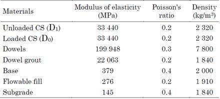
In order to validate the model and modeling techniques a heavy impact deflectometer (FWD) test was simulated, therefore, a uniform pressure of 3.2 MPa was applied for 20 ms over a 300 mm diameter contact area near the transverse joint (Figure 2). Model validation was performed by comparing the deflections and load transfer efficiency (LTE) of the FE model against the results from Westergaard's analytical edge deflection equations and FWD field measurements. It is worth mentioning that the simulation was performed with a 2-core Intel Celeron with 3.5 GHz and 6 Gb of RAM and the calculation time was approximately 4 hours. The validation is presented in Table 2, as well as the difference between the calculated deflection and the field measurement (error column). In this table, it is observed that the FE model deflections were close to the field measurements at both D0 and D1, moreover, the FE model deflections were more accurate than those calculated using the Westergaard equations. The LTE of the FE model was similar to that measured in the field (3.4 % higher) and to that calculated with the Westergaard equations (2.1 % lower).
Table 2 Validation of the PCCP FE model
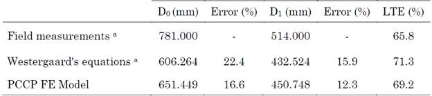
Note: LTE = D1 / D0 *100. a Based on [25]
Source: Created by the author.
Even though the FE model deflections were not accurate to the field measurements, the differences exhibited (16.6 % and 12.3 %) were acceptable considering the high variability of the field measurements, even in the literature, maximum differences of 15 % and 20 % have been accepted in pavement validations [28], [35]. Therefore, the FE model can acceptably predict the responses of a PCCP and can be used to create a direct ACP-PCCP transition.
2.2. Direct ACP-PCCP transition FE modeling
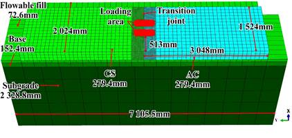
The following modifications were made to the PCCP model to create the direct ACP-PCCP transition: D1 and the dowels were removed; the flowable fill was extended along the model above the base layer; an AC layer was added, being assumed as linear viscoelastic; and due to the model and load symmetry, the symmetry boundary condition in the YZ plane was added to decrease the model size by half and reduce the computational demand, in this sense, the model consisted of 31 487 elements and 38 682 nodes and the computational time was approximately 3 hours. The properties of the other materials and characteristics of the model such as mesh size, layer thicknesses, friction between layers, and boundary conditions were retained (Figure 3). It is worth mentioning that some of the changes introduced were made to meet the thickness limits for CS or AC (200 mm to 280 mm) and flowable fill (30 mm to 500 mm) of the TransMilenio pavement [36].
2.2.1. Linear viscoelastic (VEL) properties
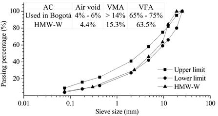
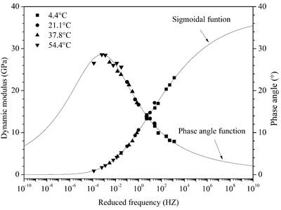
Linear viscoelasticity allows describing the AC responses under different temperature and loading frequency conditions, in addition, it allows obtaining greater accuracy in the results of FE simulations [28]. The dimensionless coefficients of the Prony series of shear modulus and relaxation times are the parameters needed to describe the VEL properties of AC (1), therefore, they were calculated from a dynamic modulus test taken from the literature, the test was performed on a 19 mm NMAS AC (HMW-W) by AASHTO TP62 - 07[37]. The dynamic moduli and phase angles of HMW-W were used since the limits for the gradation and design voids of the AC used in Bogota were well met. (Figure 4), and also because HMW-W used asphalt with a penetration grade 60/70, the same as that used in the AC in Bogotá [37], [38].
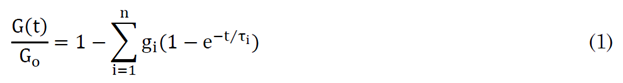
Where G(t) is the relaxation shear modulus; Go is the instantaneous shear modulus; giare the dimensionless coefficients of the Prony series of the shear modulus, τi is the relaxation time and, t is the loading time.
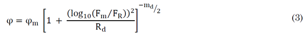
The dynamic modulus and phase angle master curves were constructed using the sigmoidal function (2) and phase angle (3), respectively, these functions allow prediction of the dynamic modulus and phase angle at experimentally unavailable frequencies. In addition, the time-temperature superposition principle was applied, which allows shifting the experimental data at different temperatures to a reference temperature as a function of the reduced frequency [39]. In this sense, the horizontal displacement factor was calculated with the Arrhenius equation, which was implicit in the reduced frequency (4). The reference temperature to construct the master curves was 25 °C since it is the maximum ambient temperature reached in Bogotá. The Microsoft Excel Solver tool was used to reduce the error between the dynamic moduli and experimental phase angles and those predicted with the functions, in this sense, the following fitting parameters were calculated, δ: -1.8265, α: 6.4003, γ: 0.3232, β: -2.3531, ΔEa: 160 991.5413, Rd: 3.9993 and md: 2.1186. Figure 5 illustrates the dynamic modulus and phase angle master curve constructed for HMW-W; it is observed the excellent fit of the experimental data in the master curves.
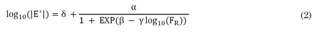

Where |E*| is the dynamic module FRis the reduced frequency in Hz; α and δ are the upper and lower limit of the sigmoidal function, respectively; β and γ are shape parameters.
Where φ is the phase angle in degrees; φmis the maximum experimental phase angle; Fmis the frequency where φmoccurs; FRis the reduced frequency in Hz; Rdand mdare shape parameters.
Where FRis the reduced frequency in Hz; F is the experimental frequency in Hz; ∆Ea is the activation energy; R is the universal gas constant, 8.314 J/(°K-mol); and T and Toare the experimental and reference temperature in °K, respectively.
From the sigmoidal function, phase angle function, and considering the parameters in Table 3, dynamic moduli and phase angles were predicted for frequencies between 10-12 Hz and 1012 Hz in order to capture the viscoelastic response of HMW-W over a wide range. The predicted dynamic moduli were converted to shear dynamic moduli [|G*|=|E*|/2(1+μ)] assuming a constant Poisson's ratio of 0.35 and then the storage and loss shear moduli were calculated and fitted to (5) and (6), respectively. The Microsoft Excel Solver tool was used to reduce the error between the calculated and predicted storage shear modulus. From the fit, 25 parameters gi and τ i , and G o were determined (Table 3), it should be noted that these parameters are mathematically equivalent to those in (1) [40]. Further details of the procedure for determining the parameters gi, τ i and Go can be found at [39], [41].
Table 3 Dimensionless Prony series coefficients and relaxation times
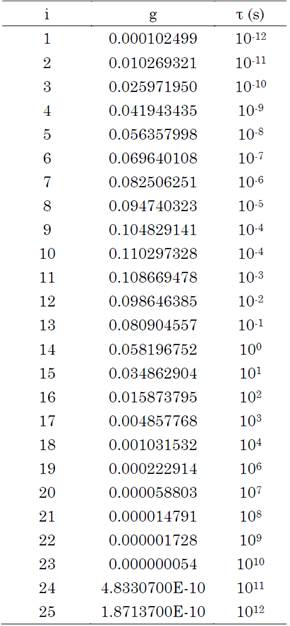
Note: Go = 13 480.25839 GPa
Source: Created by the author.
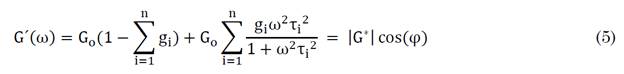
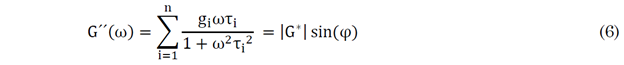
Where, G'(ω) and G´´(ω) are the storage and loss shear modulus, respectively; giare dimensionless shear modulus coefficients, τiis the relaxation time, Gois the instantaneous shear module, and ω=2πf is the angular frequency.
Figure 6 illustrates the storage and loss shear moduli of HMW-W, although it is observed under-fitting between the predicted and calculated loss shear moduli was the best fitting achieved because the fitting considers the 25 parameters giand τi, and Go simultaneously making it a little difficult to obtain a satisfactory result [39].

2.2.2. AC-concrete interface bonding
Interface bonding between AC and concrete is influenced by several factors such as dosage and type of tack coat at the interface, the type of AC, the concrete surface texture, and the temperature [11]. In addition, interface bonding plays an important role in the mechanical AC responses in composite pavements. For instance, it was established that the critical AC deformations vary significantly with inadequate tack coat application and temperature increase and, consequently, the pavement service life could deteriorate, moreover, it was established that a Coulomb-type friction model can acceptably characterize the AC-concrete interface [13]. In addition, it was showed that the maximum tensile strain at the bottom of the AC layer increases with the reduction of the COF between AC and concrete (bond decrease), therefore, poor bonding of the AC-concrete interface may reduce the pavement service life [15]. In this sense, in this study, it is believed that the AC-concrete interface bonding variation might affect the mechanical AC responses in the direct ACP-PCCP transition, thus, the Coulomb-type friction model was used to characterize the AC-concrete interface. As the interface bonding is influenced by several factors, experimentally determining COFs considering different dosages and types of tack coat can be extensive, therefore, different CFs (0.02, 0.1, 0.7, 1.5) were used to simulate different bonding conditions, from an almost frictionless case to one representing adhesion of the surfaces. However, to determine the appropriate COFs to characterize the AC-concrete interface, an FWD test was simulated for each COF and the vertical displacements and LTE were compared. This test was also simulated on a PCCP to use its results as a reference. The PCCP was created from the model in Figure 3. The CA layer was removed from the model and replaced by a CS with the same properties as the original slab in the model, and dowels were added at the transverse joint.
2.2.3. Tire-pavement contact pressure and moving vehicular loading
The vertical and tangential tire-pavement contact pressure were considered in the FE model; however, they were taken from the literature since the contact pressures of BRTs such as those used in Bogota are not reported. The contact pressures used were measured in the field on a dual-tire assembly (DTA) type 275/80R22.5 at different inflation pressures and tire loads [42]. The vertical contact pressure (PV) chosen was the one measured for the 62.1 Kn load since the rear axle tires of BRTs in Bogotá exert a similar load when operating at maximum passenger capacity [43]. The inflation pressure chosen was 552 KPa since it caused the maximum PV. The longitudinal tangential contact pressure (PL) and transverse contact pressure (PT) were 35 % and 40 % of the PV, respectively, according to field measurements at the DTA.
Figure 7 illustrates the variation of tire-pavement contact pressure along the tire footprint (Y-direction), which is based on field measurements [42]. The PV and PL were normalized to the maximum PV (1.05 MPa). The PT was not plotted, nevertheless, this pressure was equivalent to 40 % of the PV. In this study, it was assumed that the tire-pavement contact pressures of the 275/80R22.5 DTA are similar to those exerted by a BRT. Moreover, the dimensions of the DTA footprints are based on field measurements [41].
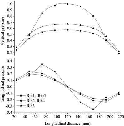
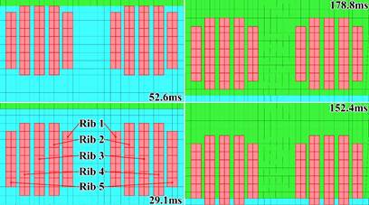
Each tire was composed of 5 treads, the outer and inner treads have been meshed with 14 and 18 elements, respectively (Figure 8). The PV, PL, and PT were assigned to each element within the treads depending on their location in the longitudinal distance.
Source: Created by the author.
Figure 8 Footprints position for the first 2 and last 2 instants of time
The mechanical response of the AC is time-dependent and in practice, this time is related to the vehicle speed, for instance, at low speeds (high loading time) the dynamic modulus is reduced and therefore higher strains are experienced compared to higher speeds [34], [44], in this sense, the tires moved at low speed (7 km/h) over a loading area with a length of 523.9 mm (Figure 3). It should be noted that the current loading area length (tire path) may cause the movement of the vehicle load to be not accurately represented. In the literature, it is mentioned that 1 m of tire path is adequate [45] therefore increasing the path was the most convenient, however, the computational cost was high, being the RAM the major limitation since increasing the length of the loading area demands a fine meshing that must be performed along the path causing an increase in the number of finite elements in the model, demanding more memory and computation time. This is an aspect that can be improved in future studies. Dynamic/implicit analysis was used to simulate vehicular movement. The simulation consisted of advancing the tire footprints over the loading area 2 elements per step, a total of 6 steps were used (Figure 8). The duration of the load in each step was calculated depending on the speed and length of the 2 elements (Duration = Length/Speed). At the beginning of the simulation, the footprints were supported on the AC at 46 mm from the transition joint, during the simulation the footprints were moved above the loading area, and in the last step, the footprints were supported on the CS at 20 mm from the transition joint.
3. RESULTS AND DISCUSSION
3.1. Effect of COF on vertical displacement and LTE
Figure 9 illustrates the effect on vertical displacement and LTE caused by varying the COF at the AC-concrete interface. The effect was measured by the FWD test. According to the results, COFs of 0.02 and 0.1 represented debonding of the AC-concrete interface since sliding was experienced at the joint between the AC and the CS causing vertical displacement in different directions. The CS (loaded) was displaced downward causing an uplift of the flowable fluid fill, and consequently, upward displacement of the AC (unloaded). Due to debonding of the interface LTE across the transition joint was not experienced (negative LTE). Furthermore, increasing the COF from 0.02 to 0.1 (increasing the bonding) caused the reduction of the vertical displacement in the AC and CS, however, this effect was negligible on the LTE since it remained negative. In this sense, COFs of 0.02 and 0.1 could represent a state of a very poor and poor bond of the AC-concrete interface, respectively.
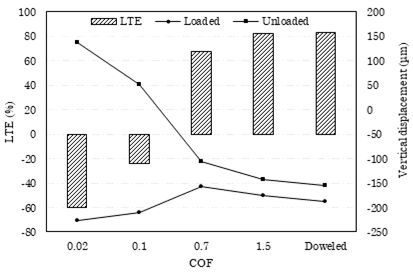
On the other hand, COFs f 1.5 and 0.7 allowed load transfer across the joint. The LTE experienced was 82.2 % and 67.1 %, respectively. In this regard, increasing the AC-concrete interface bonding increases the LTE, but increasing the interface bonding increased the vertical displacement of the AC and the CS by approximately 11 %. However, when comparing the PCCP results against those of the direct ACP-PCCP transition, for the 1.5 COF, good agreement was observed in the LTE (0.9 % difference) and the vertical displacement of the loaded (6.8 % difference) and unloaded (7.8 % difference) slab. Therefore, COFs of 1.5 and 0.7 could represent a state of good and acceptable bonding of the AC-concrete interface, respectively. Since the COFs of 0.02 and 0.1 represented debonding of the AC-concrete interface, these were not used to simulate the moving vehicular loading at the direct ACP-PCCP transition, instead, only the CFs of 1.5 and 0.7 were used.
3.2. Differential surface displacement of the transition joint
The vertical and longitudinal displacement was measured at the surface edge of the AC and CS, along the transition joint (X direction). The difference between the displacement of the AC and CS represents the differential displacement (DD). It is thought that DD can affect the performance of an ACP-PCCP transition [2], therefore, it was analyzed in this study.
Figure 10 illustrates the vertical DD, noting that for the COFs of 0.7 and 1.5, in the time instants when the tires were mainly supported on the AC (29.1 ms and 52.6 ms), the maximum vertical DD was experienced, On the contrary, when the tires were mainly supported on the CS (152.4 ms and 178.8 ms) the vertical DD was approximately 35 % lower than the maximum vertical DD. This could be caused mainly by the difference in stiffness between the AC and the concrete since the modulus of the concrete is high compared to the AC allowing for smaller displacements. As the tires advanced above the joint (78.99 ms to 131.79 ms) the tire-pavement contact pressure was progressively distributed in the CS leading to the progressive reduction of the vertical DD.
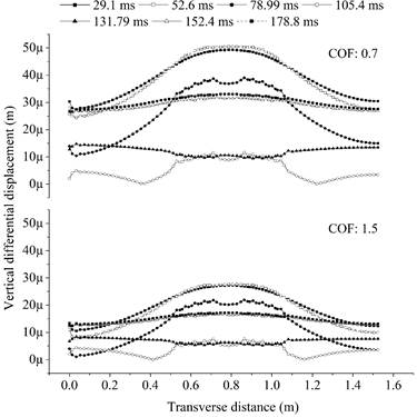
On the other hand, just below the tires, the highest vertical DD of the joint was experienced (at all time instants), since the vertical DD increased between 0.5 m and 1.1 m, the distance where it was located to the loading area. In addition, increasing the CA-concrete interface bond reduced the vertical DD by approximately 47 % at each time instant, therefore, increasing the interface bond may be conservative.
Figure 11 reveals that the difference in stiffness between the AC and the concrete also affects the longitudinal DD of the joint, since the maximum DD occurred at the instant when the tires were mainly supported on the AC (78.99 ms), in the following time instants (105.4 ms to 178.8 ms) the maximum longitudinal DD was reduced between 17 % to 61 % when the tires were mainly supported on the CS.
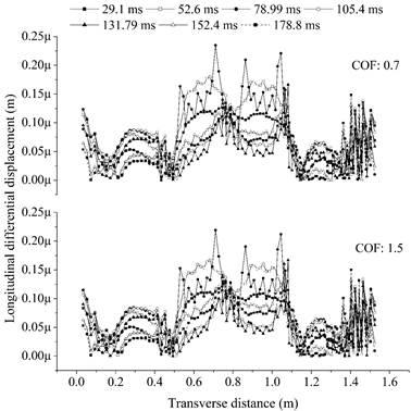
Even though longitudinal DD was about 0.5 % of the maximum vertical DD (almost negligible), the longitudinal DD may increase due to the cyclic vehicle traffic. On the other hand, increasing the AC-concrete interface bonding reduces longitudinal DD, though not significantly, since increasing the COF from 0.7 to 1.5 caused approximately a 9 % reduction of the longitudinal DD at each time instant. It is worth mentioning that the data in Figure 10 presented dispersion due to its low magnitude and the vertical scale used for visualization.
3.3. Tensile strains at the bottom of the AC
Figure 12 illustrates the longitudinal and transverse tensile strains at the bottom of the AC (εL and εT, respectively). These strains were analyzed since they are related to fatigue cracking [29]. In addition, they were also calculated for an ACP to contrast them against those of the direct ACP-PCCP transition. To model the ACP, the AC and CS in the direct ACP-PCCP transition were replaced by AC with the VEL properties in Table 3.

According to Figure 12, the direct ACP-PCCP transition might not develop cracking at the bottom of the AC, or its development might be delayed since the maximum εL in the ACP (51με) was reduced to one-third in the direct ACP-PCCP transition (16.9 με). On the other hand, even though the maximum εT (23.5 με) at the direct ACP-PCCP transition was about 2 times higher than that of the ACP (12.5 με), its magnitude was 50 % lower than the maximum εL at the ACP, therefore, the increase in εT was negligible. Furthermore, increasing the AC-concrete interface bonding might be conservative for fatigue cracking, since increasing the COF from 0.7 to 1.5 reduced the εL and εT by 6 % and 9 %, respectively. It is worth noting that the maximum tensile strains were experienced at 52.6 ms, when the tires were supported on the AC, near the edge of the joint (Figure 8).
3.4. Near-surface shear strains of the AC
The near-surface vertical shear strains are related to top-down cracking of the AC[29], therefore, the shear strains in the YZ and XZ planes were analyzed and compared against those experienced in an ACP. Figure 13a shows that the shear strain in the YZ plane (εYZ) is susceptible to the sudden change from AC to concrete since when compared to that of the ACP, the εYZ at the beginning of the simulation was up to 80 % lower, however, as the tires passed over the joint the strain progressively increased until it reached its maximum magnitude (-103 με). In this regard, the AC may experience premature near-surface cracking since the maximum εYZ was 2.7 times greater than the maximum experienced in the ACP (- 38με). The maximum εYZ happened when the tires were supported at the AC and mainly at the CS (152.4 ms). On the other hand, the effect caused by increasing the AC - concrete interface bonding was negligible, since increasing the COF increased the maximum εYZ by 1.1 %. At times between 29.1 ms and 105.4 ms, increasing the bonding reduced the εYZbetween 11 % and 29 %.
Figure 13b allows observing that the effect on the shear strain in the XZ plane (εXZ) caused by the sudden change from AC to concrete and the increased AC-concrete interface bonding was not significant since the maximum εXZ was 1.6 % lower than the maximum εXZ (61 με) in the ACP and increasing the COF reduced the εXZ by approximately 2 %. On the other hand, it is important to mention that the maximum εYZ and εXZ were exhibited just below the tires.
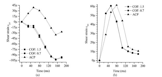
Figure 14 shows that up to 40 mm below the AC surface, the εYZ was 2.6 to 3 times higher than that of the ACP. At the direct ACP-PCCP transition and ACP, the εYZ gradually increased within the thickness until it reached its maximum magnitude at 40mm below the surface. The maximum εYZ was approximately 1.5 times greater than the surface εYZ. At depths greater than 40 mm the εYZ gradually decreased.
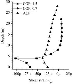
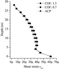
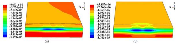
Therefore, premature near-surface cracking may initiate in the upper 40 mm of the AC. On the other hand, the effect on the εYZ caused by increasing the AC-concrete interface bonding was not significant in the upper 40 mm of the AC since increasing the COF caused between 1.1 % and 1.8 % increase in the εYZ. Figure 15 shows that the effect on the near-surface εXZ that causes the sudden change from AC to concrete, and the increase AC-concrete interface bonding might be negligible since the maximum εXZ of the direct ACP-PCCP transition was similar to that of the ACP (difference of 1.3 %), furthermore, up to 40 mm below the surface the difference between the εXZ of the direct ACP-PCCP transition and that of ACP ranged between 1.3 % and 3.3 % and, increasing the COF caused a reduction of the εXZ between 0.2 % and 1.2 %. The εXZ decreased with increasing depth in the AC, even though at depths greater than 40 mm the εXZ was approximately 15 % greater than that of the ACP, this increase may be depreciable due to its low magnitude compared to the maximum εXZ.
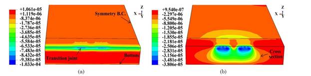
The contours of εYZ within the AC at 152.4 ms are illustrated in Figure 16. It is observed that the sudden change from AC to concrete is not conservative for the AC near the joint surface due to the relatively high εYZ experienced. In this regard, in the ACP the εYZ was rapidly reduced in the X direction, e.g., at 60 mm from the outer rib the εYZ decreased to - 1.3με (3.4 % of the maximum εYZ), on the contrary, at the transition joint at 60 mm from the outer rib, the εYZ decreased to - 65 με (63 % of the maximum εYZ), this strain was 1.7 times greater than the maximum εYZ of the ACP and, at distances greater than 60 mm the εYZ was not less than -61 με (1.6 times greater). Thus, premature near-surface cracking may also be developed along the joint.
Source: Created by the author.
Figure 16 Contours of εYZ in the AC (a) COF: 1.5 at 152.4 ms and (b) ACP at 52.6ms
Figure 16 also illustrates that even near the joint the AC experiences relatively high εYZ, for instance, the maximum εYZ measured at 72 mm from the joint just below the tires was 1.6 times higher than the maximum εYZ in the ACP (Figure 17a). Even though the εYZ (37.6 με) at 122 mm from the joint was reduced, it was similar to the maximum εYZ in the ACP. Therefore, the AC may experience premature near-surface cracking to an extent of 122 mm from the transition joint mainly below the tires. Finally, it should be considered that poor compaction near the joint could also contribute to premature cracking of the AC.
3.5. Compressive vertical strain on the subgrade top
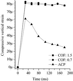
The vertical compressive strain on the subgrade top (εZ) was analyzed since it is related to rutting development. According to Figure 18, in the direct ACP-PCCP transition, premature rutting might occur since the maximum εZ was about 1.26 times higher than that of ACP. Even though later the maximum εZ decreased by about 5 %, at the end of the simulation, the εZ was 3.1 times higher than that of the ACP. On the other hand, the effect on the maximum εZ caused by increasing the AC-concrete interface bonding might be negligible since increasing the COF reduced the maximum εZ by approximately 2 %. Furthermore, when the tires were mainly supported on the CS, no variation of εZ was observed with increasing COF.
3.6. Tensile stresses in the CS
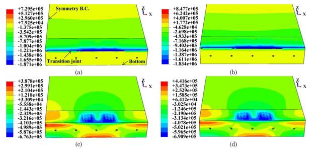
Longitudinal (σL) and transverse (σT) stresses were analyzed since cracking can develop when they exceed the tensile strength of the concrete. Figure 19a and Figure 19b illustrate σL and Figure 19c and Figure 19d illustrate σT where positive indicates tensile stress and negative indicates compressive stress. As expected, compressive stresses were experienced mainly at the CS surface below the tires, however, at depths greater than 60 mm from the surface, the σL and σT changed to tension.
Source: Created by the author.
Figure 19 Longitudinal stress contours (a) COF: 1.5 and (b) COF: 0.7, and transverse stresses (c) COF: 1.5 and (d) COF: 0.7 in the CS, at 152.4 ms (Stress in Pa). Source: Created by the author.
The maximum tensile σL and σT were around 0.27 MPa and 0.39 MPa, respectively. In this study the concrete had a tensile strength of 4.1 MPa [25], therefore, the simulated vehicular loading could not cause cracking of the concrete due to the wide difference between the concrete strength and the measured stresses. On the other hand, it was observed that increasing the AC-concrete interface bonding reduced the maximum tensile σL and σT by 3 % and 1.6 %, respectively, however, this effect might be negligible due to the low magnitude of the reduction.
4. CONCLUSIONS
The mechanical responses of a direct ACP-PCCP transition under moving vehicular loading were determined by dynamic FE analysis in order to identify failure mechanisms. In this study, COFs of 1.5 and 0.7 were used to represent good and acceptable AC-concrete interface bonding during the simulations. Lower COFs represented interface debonding. The mechanical responses of the direct ACP-PCCP transition were compared against those of an ACP. The failure mechanisms identified were: (1) near-surface shear strain of the AC (up to 40mm below the surface) with magnitude 1.6 to 3 times greater than that of the ACP mainly at the joint and below the tires, even though this strain was significant up to 122 mm from the joint, therefore, premature near-surface cracking of the AC may happen mainly near and along the joint; (2) compressive vertical strain on the subgrade top with magnitude 1.26 to 3.1 times greater than that of the ACP which might cause premature rutting; and (3) vertical differential displacement at the joint surface related to the difference in stiffness between the AC and the concrete and which could affect the pavement performance mainly under the tires. On the other hand, it was established that the tensile strains at the bottom of the AC might not cause cracking or delay its development since the strains were up to 50 % smaller than those of the ACP. In this study, the tensile stresses in the CS were also analyzed and compared against the concrete tensile strength, in this regard, it was determined that the CS could not develop cracks due to the wide difference between the concrete strength and the measured stresses. In addition, increasing the AC-concrete interface bonding might be (1) conservative on the tensile strains at the bottom of the AC and vertical differential displacement since it allows reducing the magnitude of the response, and (2) negligible on the near-surface shear strain of the AC, compressive vertical strain at the subgrade top, and tensile stresses in the CS since it does not cause a significant variation in the magnitude of the response.

