English (pdf)
 Article in xml format
 Article references
 Send this article by e-mail
 Cited by SciELO
  Cited by Google
  Similars in
SciELO
Similars in
SciELO  Similars in Google
 Permalink
INTRODUCTION
In the last decade, the development of apps for mobile devices on Android platform, along with the increase of processing velocity and storage capacity, have originated user- service oriented technologies. This is especially evident in the case of specialized user needs. An increase of software development for mobile devices to solve specific problems in business (m-business), marketplace (m-commerce), and education (m-learning) has been observed (Gasca, Camargo, & Medina, 2013) (Yin, Weng, & Chu, 2012).
Educative Software Engineering (ESE) classifies these computational tools into algorithms and heuristics. Algorithms pose different systematic processes that lead the student to a determined answer. On the other hand, heuristic tools lead to appropriation of knowledge by means of experimentation and autonomous discovering. Synergies between both algorithmic and heuristic tools produce the intelligent tutorial systems development (Galvis A., 1992).
Therefore, the aim of this paper is to present the development of a mobile app in Android platform that calculate Darcy's friction factor, to be used as a tool in both learning and professional processes. JavaScript source code for Android v. 4.0 or higher was used. Poiseuille model was used for laminar flow cases, and Colebrook-White model for turbulent flow cases. Transition zone between the two types of developed flow regimen, where flow present an unstable behavior, was also calculated.
Friction coefficient
According to regulation for potable water and basic sanitation (RAS 2017), hydraulic calculation for pressured systems in Colombia must be effectuated using Darcy-Weisbach 1845 model. It is a widely known empiric equation that determines load loss due to energy dissipation in the form of friction. This friction is the result of the interaction between fluid and its conducing structure, or pipeline (equation (1)).
Where, h f : load loss (m); f: friction coefficient; L: pipe length (m); D: pipe diameter (m); V: flow velocity (m/s); g gravity acceleration (m/s2).
There are numerous models to calculate Darcy's friction coefficient, or friction factor. Most of them are empirical models limited to the range of experimentation in which they were formulated, such as Moody equation. Another example is Swamee-Jain general equation. It presents satisfactory results for most flow conditions, except for smooth turbulent flow, in which a correction factor is necessary (Andrade, 2001).
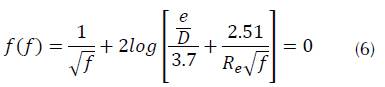
However, Colebrook-White model has been widely preferred due to its precision within turbulent conditions. Since it is a non-explicit expression, its solution requires the use of numeric methods. In this work, we used Newton-Rapson method for optimizing point integration (equation (2)).
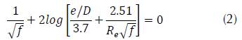
Where, f: Friction coefficient; e: pipe rugosity (m); D: pipe diameter (m); R e : Reynolds Number.
Laminar Flow
Laminar Flow is determined by values of Reynolds number below 2300. It is known that under this flow condition, viscous forces are significant in comparison to inertial forces, and therefore the fluid moves in an overlapping form with independent layers. In this case, the system behaves according to the Newton equation for viscous fluids. (Saldarriaga, 2007).
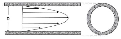
In figure 1, we see the typical velocity distribution of a laminar flow inside a cylindric pipe. The highest velocity is reached in the center of the tube, and the lowest flow velocities are found in the surface of the pipe, where the fluid is in direct contact with the solid walls. The result of this phenomenon is a parabolic velocity profile. (Saldarriaga, 2007).
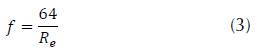
In the condition of a laminar flow, and therefore a Reynolds Number below 2300, friction coefficient may be calculated from Poiseuille equation (equation (3)).
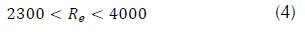
According to Reynolds' early experiments, for values between 2300 and 4000, approximately, the flow undergoes a transitional behavior. Because of that, this range of values of Reynolds Number is known as the Transition Zone. In this case, neither laminar or turbulent flow are well defined, and thus friction factor cannot be calculated (equation (4)).
Turbulent Flow
Turbulent flow may be defined as a vectoral chaos; in it we find continuous mixture conditions, due to vortex rupture. (Sotelo, 1997). Despite this widely observed phenomenon, recent studies have found vortex behavioral patterns in turbulent systems, which may defy the paradigms of turbulence according to current notions. In fact, tests to model disorganized and complex turbulent flow conditions into series of somehow organized movement patterns, known as "coherent structures", have been made with mixed results. (Dennis, 2015).
Newton-Raphson Method
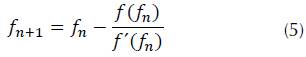
Newton-Raphson method optimizes the Newton point integration method by defining a more robust convergence equation. Convergence will exist if the difference of absolute value of calculated values in two successive iterations decreases while the number of iterations (n) increases (Quinta & Villalobos, 2005). The algorithm has been generalized in numerous forms to solve non-linear problems, equation systems, non-linear differential, and integral equations (Díaz & Benítez, 1998). However, if the function is not differentiable and presents discontinuity in the calculation interval, the Newton-Raphson method will not converge. In such cases, it will be necessary to apply another numeric method to find the root of the non-linear equation. Newton-Raphson method requires an initial assumed value f 0 (seed value) (equation (5)).
Now, in the problem of calculating the friction factor, Colebrook-White equation becomes the function, as noted below (equation (6)).
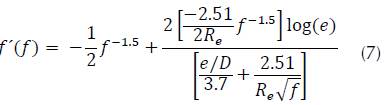
And, the first derivative becomes (equation (7)).
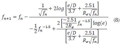
Therefore, Newton-Rapson convergence equation will become (equation (8)).
METHODOLOGY
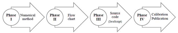
In this work, we followed four main methodological steps (figure 2): (1) to define the numeric method to solve Colebrook-White equation in the Turbulent Flow condition, (2) to stablish the flow diagram of the app's iterative process, (3) to develop the source code in JavaScript, and (4) to calibrate resulting calculations with Goal Seek function in Excel.
Source code was developed using JavaScript. Once the solution converges, the result appears in a separated window on the screen. The relative rugosity and Reynold Number, which are both dimensionless.
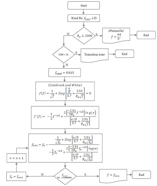
In figure 3, we present the flow diagram of the iterative process the app follows to calculate Darcy's friction factor.
RESULTS
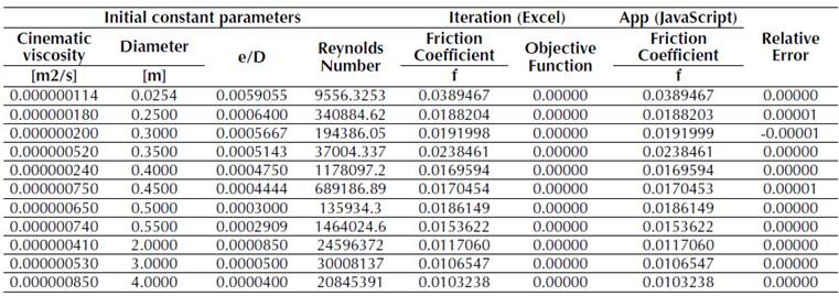
Resulting calculations for Darcy's friction factor were calibrated by comparing them to solutions calculated through the Goal Seek function in Excel. In table 1, we present the comparison between various calculation with different input data.
Laminar flow conditions
The relative rugosity of a pipe is 0.0000015. If the Reynolds Number is 1550, the app conduces the calculation of friction coefficient using Poiseuille model for Laminar Flow. Therefore, the result will be f = 0,0412903, as shown in figure 4.

Transition zone flow conditions
If the relative rugosity of the pipe is 0.0000045 and the Reynolds Number is 3456, the flow is in the transition zone, so the app will indicate exactly that as shown in figure 5.

Turbulent flow conditions
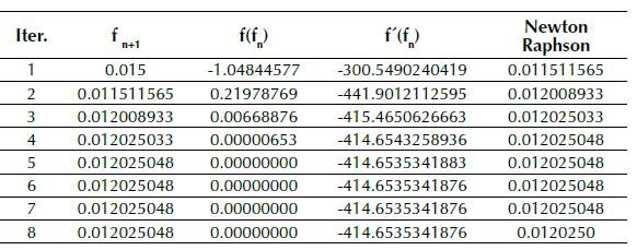
If the relative rugosity of a pipe is 0.0000018 and the Reynolds Number is 845203, the app will use Newton-Raphson method to solve Colebrook-Whi-te equation and calculate the friction coefficient. Seed value is already determined to f= 0.015. the result is f = 0,0120250, as shown in figure 6.

The solution for turbulent flow conditions is coherent with the one obtained by the Goal Seek function, shown in the table 2.
CONCLUSIONS
The app "App cálculo del coeficiente de fricción" accurately calculates Darcy's friction factor for Laminar and Turbulent Flow Conditions. It also indicates when the input data corresponds to the Transition Zone.
The development of mobile apps for educational purposes (m-learning) is a valuable tool for autonomous learning. Therefore, the app "App cálculo del coeficiente de fricción" contributes to Fluid Mechanics and Hydraulics academical environments. It allows students to experiment with varied input data and explore different initial conditions of the problem.