


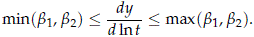
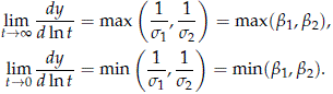
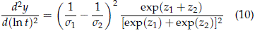
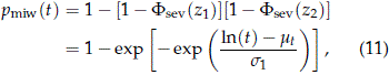
Services on Demand
Journal
Article
 English (pdf)
 Article in xml format
 Article references
 Send this article by e-mail
Indicators
-
 Cited by SciELO
 -
 Access statistics
Related links
-
 Cited by Google
 -
 Similars in
SciELO
Similars in
SciELO -
 Similars in Google
Share

 Permalink
Revista de la Academia Colombiana de Ciencias Exactas, Físicas y Naturales
Print version ISSN 0370-3908
Rev. acad. colomb. cienc. exact. fis. nat. vol.38 no.148 Bogotá July/Sept. 2014
Matemáticas
1 School of Statistics, Universidad Nacional de Colombia, Sede Medellín,
2 Experimental Statistics, Louisiana State University, * Correspondencia: Sergio Yáñez, syanez@unal.edu.co.
Recibido: 23 de junio de 2014. Aceptado: 28 de agosto de 2014
Abstract
Lifetime and survival data are usually the lives of subjects, units, or systems that has been exposed to multiple risks or modes of failure. In the analysis of the data, however, is common to ignore the modes of failure because they are unknown, they are not recorded, or because the complexity of including them in the modeling. It is of interest knowing when the conclusions might be robust to ignoring the failure modes in the analysis. In particular, it would be useful to characterize situations where it could be safely said that the modes of failure effect on the analysis would be negligible or that failing to include such information could completely invalidate the conclusions drawn from the study. As a first step in identifying when the failure modes have little or large influence on the competing risks model, this article studies two different competing risks models: (a) a model with independent risks; (b) a model derived from a multivariate Weibull with dependence.
Key words: competing risks, probability plots, log-location-scale family, Weibull distribution, multivariate Weibull with dependence, lognormal distribution.
Resumen
Los datos de tiempos de falla y sobrevivencia se refieren generalmente a la vida de individuos, unidades o sistemas que han sido expuestos a múltiples riesgos o modos de falla. Sin embargo, en el análisis de los datos es común ignorar los modos de falla porque son desconocidos, no se registran o por la complejidad de la modelación al incluirlos. Es importante, por lo tanto, determinar la robustez del análisis ignorando los modos de falla. En particular, sería útil caracterizar situaciones donde pudiera decirse que el efecto de los modos de falla en el análisis es despreciable o donde no incluir tal información pudiera invalidar completamente las inferencias del estudio. Como un primer paso para identificar cuando los modos de falla tienen poca o mucha influencia en el modelo de riesgos en competencia, este artículo estudia dos modelos de riesgos en competencia: (a) un modelo con riesgos independientes; (b) un modelo derivado de una distribución Weibull multivariada con dependencia.
Palabras clave: riesgos en competencia, gráficos de probabilidad, familia de log-localización y escala, distribución Weibull, distribución Weibull multivariada con dependencia, distribución lognormal.
1. Introduction
In the analysis of lifetimes one is usually dealing with time to an event of interest like failure of a component or system, dead of an individual, or end to a subscription service. In most cases, there are several competing reasons (risks or modes of failure) that cause the event of interest. Say, for example, that we were interested in the first time that a bicycle fails. In this situation, the competing risks for failure include: a flat tire, a broken chain, or the rupture of a brake cable.
The interest in competing risks is old but the formal development and application of the methodology to problems in engineering, survival analysis, and other applied areas is relatively new. Crowder (2001, 2012) and Pintilie (2006) provide historical accounts, relevant references, and methodology.
It is interesting that, for many years, competing risks were not in the front end of reliability and survival analysis. Beyond the statistical challenges of handling properly multiple risks in an analysis, there are, however, some compelling reason for which the competing risks might have been ignored in the analysis of the data: (a) sometimes the competing risks are hidden or unknown to the observer; (b) the competing risks may be well known but it is difficult or expensive to identify the risk that caused the event; (c) in other cases the cost and time spent on determining the failure cause ends being a waste of resources because ignoring the competing risks in the analysis is as good as the analysis that takes them in consideration. This is the case for example, with the analysis of the Shock Absorber data in Meeker and Escobar (1998) where a simple Weibull analysis, that ignores the failure modes, is basically indistinguishable of aWeibull analysis that takes in consideration the two observed failure modes.
It would be useful to have a clear understanding on the situations (e.g., model, data type, risk type) where the use of the competing risks information makes a difference in the analysis. Meeker, Escobar, and Hong (2009, page 157), in the context of a complex model and analysis, came to the conclusion that in a competing risks model with two risks that are log-location-scale distributed with similar shape parameter, the distribution of the competing risks can be approximated by the same log-location-scale distribution with a shape parameter that is in between those for the marginal distributions and that the adequacy of the approximation does not depend strongly on amount of association between the two risks. One, however, would need a formal study of the problem to provide a more definitive answer.
The purpose of this article is to study two simple competing risks models with Weibull risks to assess the effect of the risks on the time to the event of interest and the inter-relationships between the two models. This might be useful in setting a simulation study that could provide broader guidelines on the situations where ignoring the competing risks information in the analysis could lead to erroneous conclusions.
The rest of the paper is organized as follows. Section 2 is an introduction to competing risks models (CRMs) and some features of their probability plots. Section 3 discusses the competing risks model with Weibull independent risks and its characteristics. Section 4 presents a competing risks model derived from a bivariate Weibull distribution with dependent risks. Section 5 describes generalization of the results to CRMs with k > 2 risks and anticipate some of the difficulties in generalizing the results to log-location-scale families in general. Section 6 summarizes the results in the paper and outlines future related work. Section 7 contains appendixes with technical details for some of the results given in the paper.
2. Competing Risks Models and Their Probability Plots
Lifetimes of units or individuals subject to two risks (or modes of failure), k = 2, can be modeled as a seriessystem. Each risk is like a component in a series system with two components. The unit has a potential lifetime associated with each risk. The observed lifetime for the unit is the minimum of these individual potential lifetimes Ti, i = 1, 2. Informally, we refer to Ti as the Risk i and to the model as the competing risks model (CRM).
For a CRM with two risks, a quantity of interest is Tm = min (T1, T2) which has the cumulative distribution function (cdf)
where Pr(T1 > t, T2 > t) is computed with respect to the joint distribution of (T1, T2).
When the risks are independent
where Fi(t) is the cdf for Ti, i = 1, 2.
In the case of k risks, Fm(t) = 1 - Pr(T1 > t, . . . , Tk > t) for dependent risks and Fm(t) = 1 - Pki =1 Pr(Ti > t) = 1 - Pki =1 [1 - Fi(t)] for independent risks, where Fi(t) is the cdf for the i risk. See Meeker and Escobar (1998, chapter 15) for additional information.
2.1. Probability Plots and CRMs
In theoretical and applied work with lifetime data, probability plots have shown to be useful for multiple purposes, see Meeker and Escobar (1998, chapter 6) for detailed explanation on their construction, interpretation, and use. In this paper we will use probability plots to display the distribution function of the competing risks model along with the distribution of the individual risks. As illustrated later, with proper choice of the plot scales, the distributions of the individuals risks, Fi(t), show up as straight lines in the probability plot, but the CRM cdf, Fm(t), is usually a non-linear curve in the plot.
Graph of a cdf on a log-location-scale plot
Consider a log-location-scale probability plot defined by the scales [ln t, F-1(p)] where F(z) is a standardized continuous cdf that does not depend on unknown parameters, 0 < p < 1, t > 0, and ln t denotes the natural logarithm of t. It is known, see for example Meeker and Escobar (1998, chapter 6), that in these scales any cdf of the form F[(ln(t) - m)/s] (where s > 0) plots as a straight line with slope 1/s.
In a log-location scale probability plot, if a cdf F(t) is a fairly linear curve, then there is strong information that, with properly chosen (m, s), the cdf F(t) is well approximated by the distribution function F[(ln(t) - m)/s]. We will use this feature of probability plots later in studying the properties of some CRMs.
The following result considers a probability plot defined by the scales [ln t, F-1(p)] and the plot {ln t, F-1 [F(t)]} of a cdf F(t), t > 0 on it.
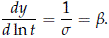
Result 1. For an absolutely continuous cdf F(t) = Pr(T ≤ t), t > 0 the slope of the curve {x = ln t, y = F-1[F(t)]} in the probability plot [ln t, F-1(p)] is given by
where f (t) and f(z) are the probability density functions (pdfs) corresponding to F(t) and F(z), respectively.
The proof of (1) follows after differentiation of y with respect to ln t.

Because t, f (t), and the function f(z) are all nonnegative, the slope in (1) is non-negative. This is the expected behavior because the cdf F(t) is a non-decreasing function of ln(t).
2.2. The competing risks model for independent positive continuous variables
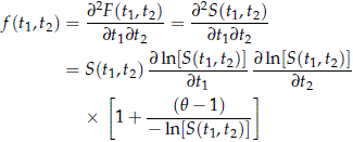
For the CRM with two independent risks, k = 2,
where Fi(t) and fi(t) are the cdf and pdf of Ti and Si = 1 - Fi(t) for i = 1, 2. Then, using (1) with F(t) = Fm(t),
The competing risks model for two independent log-location-scale continuous variables
Now suppose that the individual risks are independent and log-location-scale distributed. That is, T1 and T2 are independent, and Ti ∼ F(zi) , i = 1, 2, where
-∞ < mi < ∞, si > 0, and F(z) is a differentiable cdf that does not depend on unknown parameters. In this case,
where fi(z) is the pdf corresponding to the cdf Fi(z), i = 1, 2.
Thus for a competing risks model with two independent log-location-scale risks, the slope of the curve {x = ln t, y = F-1[Fm(t)]} in the probability plot [ln t, F-1(p)] is given by
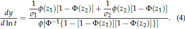
In this case, the cdfs of the individual risks Ti appear as straight lines in the probability plot. But the line corresponding to the CRM cdf is not necessarily linear. For an example, see Figure 1 which is described in the following section.
3. Competing RisksModelWith Independent Weibull Risks
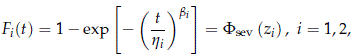
A Weibull cdf F(t) is often written as
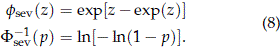
where h > 0 is a scale parameter and b > 0 is a shape parameter. Fsev(z) = 1 - exp[-exp(z)] is the standard smallest extreme value distribution, m = ln(h), and s= 1/b. When T has a Weibull distribution, we indicate it by T ∼ WEI(h, b).
Although (5) and (6) are equivalent specifications of the Weibull cdf, (5) is commonly used in engineering and (6) is convenient on theoretical developments, for numerical stability in computations, and for notational standardization with other log-location scale distributions. For additional details see Meeker and Escobar (1998) and Lawless (2003).
Then the Weibull competing risks model with two independent risks has the cdf
Figure 1 shows pmiw(t) in aWeibull probability plot with scales [ln t, F-1sev(p)]. The plot also shows, as straight lines, the cdfs for the two Weibull independent risks defining the CRM model. In this case, because the plot of pmiw(t) is non-linear, we know that the distribution of the CRM is not a Weibull distribution. For this and other figures in the paper, the model parameters values were chosen for illustration purposes.
Important properties of the CRM with independent Weibull risks
The following results characterize the CRM with independent Weibull risks.
Result 2. Consider the graph {x = ln t, y = F-1sev[pmiw(t)]} of the cdf pmiw, for the CRM with independent Weibull risks, on aWeibull probability plot. The following results hold.
(a)
- The slope of pmiw(t) in the probability plot is the convex combination
To prove this result, note that the density and the quantile functions for Fsev(z) are
Thus fsev[F-1sev(p)] = (1 - p)[-ln(1 - p)] and we get
From (3) with F(z) = Fsev(z) and f(z) = fsev(z), one obtains (7).
A more detailed proof of (7) can be obtained as the special case with q = 1 in Appendix B.1.
(b)
- When b1 = b2 = b, pmiw(t) is the cdf of a WEI(h, b) where
To prove this result, use (7) with s1 = s2 = 1/b to obtain
Thus pmiw(t) is linear in the Weibull probability plot which implies that it is a Weibull cdf. The particular form of the shape parameter is obtained from the anti-log of mt in (11) with s1 = s2 = 1/b.
The fact that, in this case, pmiw(t) is a Weibull cdf is in agreement with the following known result: the minimum of k independent Weibulls, that have a common shape parameter b but possibly differing scale parameters, is Weibull distributed with shape parameter equal to b. For details, see, for example, Meeker and Escobar (1998, page 372) and the related Result 3 below.
(c)
- The slope of the curve {x = ln t, y = F-1sev[pmiw(t)]} is bounded by (b1, b2) as follows. Using (7)
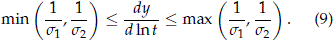
Or equivalently,
This is consistent with the observation made in Meeker et al. (2009, page 157) where they found through simulation and sensitivity work that in modeling competing risks data with a single Weibull distribution (i.e., ignoring the failure mode), the estimated Weibull shape parameter tend to fall between the two Weibull shape parameters used to simulate the data. This result suggest that the closeness between the shape parameters of the risks' cdfs might be an important factor in determining if a single Weibull model could fit well a Weibull CRM with independent risks.
(d)
- In the limit
These limiting behaviors follow directly from (7) and the relationships bi = 1/si, for i = 1, 2.
In Figure 1, as ln(t) → -∞, the distribution pmiw(t) approaches the individual risk F1(t) and also the derivative of pmiw(t) with respect to ln(t) converges toward b1. Similarly, when ln(t) → ∞, pmiw(t) approaches F2(t) and the derivative of pmiw(t) with respect to ln(t) converges toward b2.
- (e) The curve {x = ln t, y = F-1sev[pmiw(t)]} is concave when b1 ≠ b2.
To verify this result, obtaining the derivative of (7) with respect to ln t to obtain
which is positive when s1 ≠ s2. This implies that the curve (ln t, y) is concave. Because the curvature of the [ln t, y] is proportional to (10), see for example Courant and John (1965, page 357), then is also proportional to (1/s1 - 1/s2)2 = (b1 - b2)2. Note that derivative (10) is a special case of Appendix B.2 when q = 1.
Large values of (10) are associate with large curvatures of the curve (ln t, y) and we can use curvature as another criteria to help in the decision when is that a simple Weibull distribution fits well the CRM model with independent Weibull risks. In particular, a single Weibull model would fit well aWeibull CRM cdf with independent risks if the two Weibull shape parameters in the CRM model are not far apart. There are situations, however, where the curvature is large just in an interval with negligible probability content with respect to the CRM cdf, in those case the simple Weibull distribution will fit well the CRM model in an interval of high probability with respect to the CRM cdf, regardless of sizes of the scale parameters. See the discussion at the end or Result 3 for a case where the curvature is large just in an interval with negligible probability content with respect to the CRM cdf.
All the outcomes in Result 2 can be extended readily, with trivial minor changes, to a CRM with k > 2 independent Weibull risks. See Jiang and Murthy (2003) for results related to items (a) and (d) in Result 2.
CRM with independent Weibull risks and similar shape parameters
An important problem is the modeling of competing risks data when the risks are Weibull distributed with similar shape parameter. The following result considers that setting in the special case when the risks are independent.
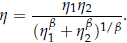
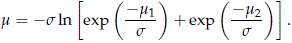
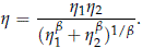
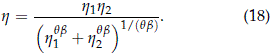
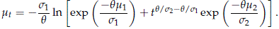
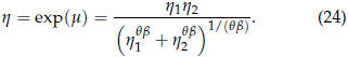
Result 3. Consider the cdf pmiw(t) of the CRM T = min(T1, T2) with independent risks. Suppose Ti ∼ WEI(hi, bi), i = 1, 2. Then when bi → b > 0, i = 1, 2, pmiw(t) converges to a WEI(h, b) cdf where h = (h1h2)/(hb1 + hb2 )1/b.
To prove this result, it can be shown that (use Appendix C with q = 1),
where
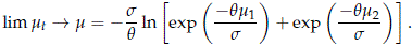
The proposed results follows after letting bi → b, i = 1, 2 (which is equivalent to si → s, i = 1, 2 where s = 1/b). Then
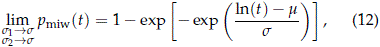
Where
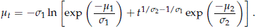
Equation (12) corresponds to a WEI(h, b), where b = 1/s, h = exp(m), with
Note that (11) is well approximated by a Weibull distribution when mt is fairly constant. That is, when mt does not depend strongly on t. Values of s1 and s2 closed to each other might have that effect on mt. Observe, however, that mt could also be fairly linear in an interval of high probability content (with respect to the CRM cdf), if exp(-m1/s1) dominates t1/s2-1/s1 exp (-m2/s2) in that interval. Or equivalently, when F1(t) > F2(t) in a interval with high pmiw(t) probability content. A similarly situation arises when the second risk is the dominant one, that is when F2(t) > F1(t) in a interval with high pmiw(t) probability content. Thus to anticipate the linearity of the CRM cdf in a probability plot, two factors emerge as important to be considered: (a) the closeness of the shape parameters and (b) the crossing point of the cdfs F1(t) and F2(t) associated with the two risks in the model. These two factors may or may not interact depending of the CRM model parameters. Extreme cases are when the crossing point is too far to the right or to the left in the plot in whose case the CRM cdf can be approximated well by a single Weibull distribution.
Next section studies a CRM derived from a bivariate Weibull distribution with dependence between the risks. We will see that the properties for the CRM model with independent Weibull risks extend to this new CRM.
4. Competing Risks Model Derived From a Bivariate Weibull Distribution
In practical application the competing risks might not be independent and the dependence can greatly complicate the statistical modeling and the data analysis, see a detailed account in Crowder (2001, chapter 7).
Here we consider a simple model that allows for positive dependence. In the analysis of lifetime data, models that allow for risks with positive dependence are reasonable because in those cases the risks are jointly leading toward shorter lives, but see Crowder (1989) for a somehow dissenting opinion.
The setting here is that the risks (T1, T2) are jointly distributed with a joint survival function S(t1, t2) = Pr(T1 > t1, T2 > t2) given by
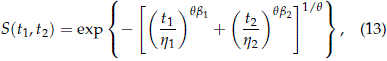
where ti ≥ 0, bi > 0, hi > 0, i = 1, 2, and q > 1. The his are scale parameters and the bis are shape parameters. q characterizes the association between the two variables. In particular, the Kendall's coefficient of association between T1 and T2 is equal to 1 - 1/q.
Johnson and Kotz (1972, pages 268-269) have an early description of this distribution. Lee (1979, pages 268-269) discusses this distribution in a larger context of multivariate distributions with Weibull properties. Kotz, Balakrishnan, and Johnson (2000, page 408) call it a Weibull form B and show how to derive it through power trans- formations of the variables from a bivariate exponential distribution. It can be shown that (13) corresponds to a Gumbel-Hougaard survival copula evaluated at two Weibull survival marginals, see Nelsen (2006, page 96). This bivariate Weibull has has been used in dependent failure-times analysis, among others, by Hougaard (1986), Hougaard (1989), and Lu and Bhattacharyya (1990).
Using the log-location scales wi = [ln(ti) - mi]/si, with mi = ln(hi), si = 1/bi, the survival distributions in (13) becomes
The joint distribution function of (T1, T2) is
where F1 (t1) and F2 (t2) are the Weibull marginal distributions of T1 and T2 given by
where the zi are as in (2).
The distribution F(t1 , t2 ) is absolutely continuous and its density is (see Appendix D)
where for i = 1, 2
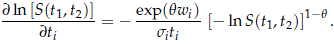
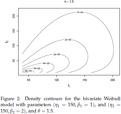
Figure 2 shows contours of the bivariate Weibull for a specific and convenient choice of the parameters. The southwest to northeast orientation of the plot is an effect of the positive dependence (q = 1.5) between the two Weibull risks. With independence, that is q = 1, and everything else being the same, the density contours will be fairly symmetric about a vertical line drawn at time t1 = 106.
The CRM derived from the Bivariate Weibull
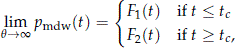
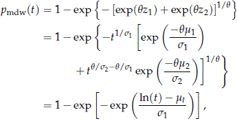
As before, using Tm = min(T1, T2), it follows that the survival function smdw (t) of Tm is
where zi = [ln(t) - mi]/si, mi = ln(hi), and si = 1/bi. The related distribution function pmdw for the CRM Tm
is
With q = 1, the pdf pmdw(t) is equal to the cdf pmiw(t) for the CRM with independent risks T1 and T2 .
Result 4. Consider the cdf, pmdw(t), given in (16). Then (see Appendix A)
- 1. For each t, pmdw(t) is a monotone decreasing function of q.
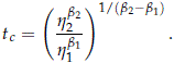
- 2. Assuming, without loss of generality, that b1 < b2 ,
where tc is the time at which the marginal distributions F1(t) and F2(t) cross. That is, the time at which z1 = z2 , or equivalently
- 3. When b1 = b2,
for all t > 0.
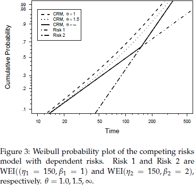
Result 4 implies that the cdf pmdw(t) of Tm , for the bivariate case with dependence, is bounded from above by the cdf pmiw of Tm in the model with independent risks and below by the marginals associated with the Weibull bivariate risks. For example, in Figure 3, the dashed line (the one closest to the northwest corner) corresponds to the CRM with q = 1. The solid line is the CRM with q = ∞. This cdf agrees with the distribution of Risk 1 for times before the time at which the two marginals cross each other and with the distribution of Risk 2 for times after that crossing point of the marginals.
Important properties of the CRM with dependent Weibull risks
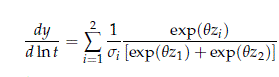
Result 5. Consider the Weibull probability plot {x = ln t, y = Φsev-1 [ pmdw (t)]} of the cdf pmdw (t) in (16) for the CRM derived from the bivariate Weibull distribution in (14). The following results hold.
(a)
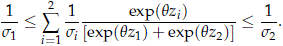
- The slope of pmdw(t) in the probability plot is the convex combination
where zi = [ln(t) - mi]/si .
To verify this result, use (15) to obtain the y-ordinate
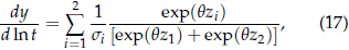
Then taking the derivative of y with respect to ln t yields (17), see Appendix B.1.
The similarity between (7) and (17) is more than a simple coincidence. We proceed to show that the CRM pmdw(t) is an extension of the CRM pmiw(t) with characteristics very similar to the pmiw(t) model. The similarities between the two models was unknown to us at the outset of this study.
(b)
- When b1 = b2 = b, pmdw(t) is the cdf of a WEI(h, b) where
With b1 = b2 = b, then s1 = s2 = 1/b and it follows from (17) that
which implies that pmdw(t) is a WEI(h, b). The specific value of h is derived in Appendix C.
It is interesting that, even in the presence of dependence, the equality of the shape parameters implies a Weibull distribution for the CRM cdf, pmdw(t).
See the related Result 6 below which shows that when the shape parameters of the risks are closed to each other, the CRM has a distribution that might be approximated by a simple Weibull distribution.
(c)
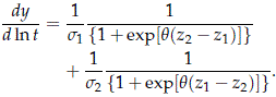
- The slope of the curve [ln t, y] is bounded by (b1, b2) as follows
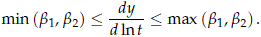
To prove this, suppose that maxi {1/si} = 1/s2 then using (17) it can be verified that
As in the case of independent risks it is useful to know that the CRM cdf has a derivative with respect to ln t that is bounded by the shape parameters of the risks defining the model.
(d)
- In the limit
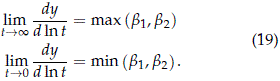
To prove this, note that if s1 = s2 the result holds in view of item (b) above. Then assume that s1 ≠ s2. If maxi {1/si} = 1/sk = bk then
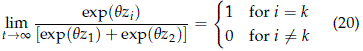
and
Using (20) and (21), when taking the limits of dy/d ln t, yield the results in (19) for the limiting behavior of the derivative function.
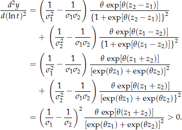
(e)
- The curve [ln t, y] is concave when b1 ≠ b2.
Taking the derivative of (17) with respect to ln t (see Appendix B.2)
Because this second derivative is positive, the concavity of the curve follows. The concavity, however, is also proportional to q and large values of q could imply large concavity and curvature of the curve even in the presence of shape parameters that are closed to each other. This is different to what happens in the independent risks case where similar shape parameters imply small concavity.
CRM with dependent Weibull risks and similar shape parameters
Result 6. Consider the cdf pmdw(t) of the CRM given in (16) and derived from the bivariate model with dependence in (14). When bi → b > 0, i = 1, 2, pmdw(t) converges in distribution to a WEI(h, b) where
See Appendix C for justification of the result.
Note that the limiting Weibull distribution WEI(h, b) was already obtained in (18) as a special case of equal shape parameters. The special case with independent risks given in Result 3 is obtained with the value q = 1.
5. Other Competing Risks Models
As noted earlier, the findings in Result 2 extend directly to a CRM with k > 2 independent Weibull risks and cdf pmiw(t) = 1 - Pki=1 [1 - Fsev(zi)], where zi = [ln(t) - mi]/si , i = 1, . . . , k.
The bivariate Weibull model described in (13) has been extended to the case of k > 2 dependent risks. In this case, the survival function is S(t1, . . . , tk) = exp { - [Ski =1 exp(qwi)]1/q}, where wi = [ln(ti) - mi ]/si. Lee and Wen (2010) derive the density and the general moments of the distribution for any integer k ≥ 2. They also apply the model to a data set with three variables. All the properties in Result 5 extend readily to the CRM cdf, pmdw(t) = 1 - exp {- [Ski =1 exp(qzi)]1/q }, zi = [ln(t) - mi ]/si, derived from this k > 2 dimensional Weibull distribution with dependent risks.
There is a large number of other Weibull multivariate models. Murthy, Xie, and Jiang (2004) provide a comprehensive collection of univariate and multivariate Weibull models and Crowder (1989) proposes an interesting multivariate Weibull model. There is not, however, assurance that the properties discussed here are satisfied by those models. For other models of interest, their properties need to be studied separately.
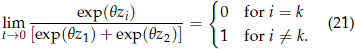
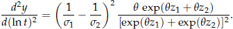
A natural inquire is if the results presented here extend to the CRM model derived from log-location-families. We have not studied this in detail, but the items in Result 2 do not extend in their full generality to a CRM derived from a log-location-scale family. This was surprising and unexpected to us. For example, suppose Ti ∼ LOGNOR(mi , si), i = 1, 2 with T1 and T2 independent. As before Tm = min(T1, T2). Thus, Fm(t) = 1 - Fnor(-z1) Fnor(-z2) and the slope of the curve { x = ln t, y = F-1 nor[Fm(t)] } , see (4), in a lognormal probability plots is
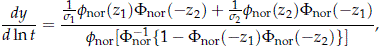
where fnor(z) and Fnor(z) are the standardized normal pdf and cdf, respectively. Figure 4 shows the slope of the curve when m1 = 5, m2 = 6, s1 = 3, and s2 = 2. Clearly,
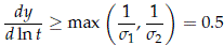
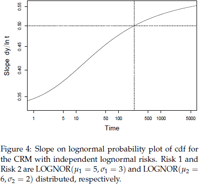
for t > 236. In contrast to the Weibull case, the slope of the Fm(t) in the lognormal probability plot is not bounded by the sis as in (9).
6. Conclusions and Future Work
The characteristics of the Weibull CRM with independent risks and the CRM derived from the bivariate Weibull with dependence are very similar. For a CRM with two risks, based on the information drawn from this work, we can say that important factors in deciding when the inference is robust to ignoring the failure mode include: (a) the relative sizes of the Weibull scale parameters; (b) the crossing point of the marginal distributions; and (c) the size of the dependence among the factors.
Similar conclusions apply to the models with k > 2 risks considered here. A single Weibull model might describe the CRMwell if: (a) the ratio between the largest and the smallest shape parameters is small and the dependence among the risks is not large; or (b) there is a dominant risk.
It is plausible that these continue to be important factors when studying the CRM for other distributions, but additional work is needed to corroborate these preliminary findings.
There is need to study other distributions beside the Weibull and the lognormal and to consider other situations with dependent risks. The brief look into the lognormal case indicates that caution should be exercised when trying to generalize the conclusions to other distributions because the results do not seem to be completely generalizable to other competing risks situations of interest like CRMs derived from general log-location-scale families.
Eventually, the model robustness problem will have to be addressed using meaningful and well formulated simulation studies with complete, dependent, and censored data. Toward that end, the results of studies like the one pursued here would be useful because a good understanding of the important factors in a model facilitate the test planning and the interpretation of a simulation study.
Acknowledgments
This work was supported by Colciencias, Colombia. This is part of the research project "Characterization of Dependence in Competing Risks Models in Industrial Reliability Data," code 110152128913. This project is directed by Sergio Yáñez, Luis Escobar, and Nelfi González.
7. Appendixes
A. Monotonicity of the CRM cdf pmdw(t) as a function of q
From (15), smdw(t) = exp (-R1/q), where R = exp(qz1) +exp(qz2), and zi = (ln(t) - mi)/si, i = 1, 2.
Consider
Note that ln(R) = ln[exp(qz1) + exp(qz2)] > ln[exp(qzi)] = qzi , for i = 1, 2. Thus for fix t, [j ln(R1/q)/jq] < 0. This implies that R1/q is monotone decreasing on q. Consequently, smdw(t) is increasing on q and pmdw(t) = 1- smdw(t) is decreasing on q.
B. Important Properties of the CRM
This appendix provides details of the properties of the CRM derived from the bivariate Weibull defined in (13). The correspondent properties for the CRM with independent Weibull risks are obtained by setting the dependence parameter to q = 1.
B.1. Slope of the curve {ln t, F-1sev[pmdw(t)]} in a Weibull probability plot
From the definition of fsev(z) and F-1sev(p) in (8) and using (15) and (16), we get that for 0 < p < 1,
Then with p = pmdw(t), we get
Now we compute t dmdw(t), where dmdw(t) is the density corresponding to the cdf pmdw(t) given in (16).
Direct differentiation of pmdw(t) yields
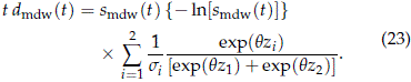
Taking the ratio between (23) and (22) and using (1), we get
which is the result suggested in (17). Note that with q = 1, one obtains the independent risks case suggested in (7).
B.2. Concavity of the curve {ln t, F-1sev[pmdw(t)]} in a Weibull probability plot
To show that the second derivative of y with respect to ln t is positive, we write
Then
For the CRM with independent Weibull risks, use q = 1. In this case the second partial derivative is still positive and takes the value suggested in (10).
C. Cdf for CRM with Weibull Dependent Risks and Similar or Equal Shape Parameters
where
When bi → b > 0, i = 1, 2, it follows that si → s = 1/b > 0, i = 1, 2, and
Thus pmdw(t) is the cdf of a WEI(h, b), where
Note that: (a) when b1 = b2 = b, pmdw(t) is the cdf of a WEI(h, b) with h given by (24); (b) when b1 = b2 = b and q = 1, pmdw(t) = pmiw(t) and they are the cdf of a WEI(h, b) with h given by (24) evaluated at q = 1. This is the CRM cdf with independent Weibull risks considered in Result 3.
D. Bivariate Density
The density is given by the mixed second partial derivative of S(t1, t2) with respect to t1 and t2. For simplicity write S = S(t1, t2) and define M = -ln(S) = [exp(qw1) + exp(qw2)]1/q . Using wi = [ln(ti) - mi]/si and taking the derivative of ln(S) with respect to t2,
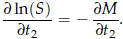
Equivalently,
Taking the derivative with respect to t1
Direct computations yield
Substituting (26) into (25)
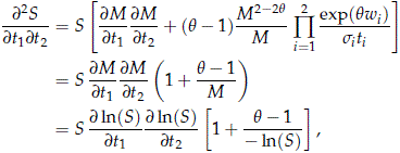
where for i = 1, 2
See Lu and Bhattacharyya (1990, page 554) for an equivalent expression for the density.
References
Crowder, M. (1989). A multivariate distribution with Weibull connections. Journal of the Royal Statistical Society. Series B (Methodological) 51(1): 93-107. [ Links ]
Crowder, M. J. (2001). Classical Competing Risks. New York: Chapman & Hall/CRC. [ Links ]
Crowder, M. (2012). Multivariate Survival Analysis and Competing Risks. New York: Chapman & Hall/CRC. [ Links ]
Courant, R. and F. John (1965). Introduction to Calculus and Analysis: Volume One. New York: Interscience Publishers. [ Links ]
Hougaard, P. (1986). A class of multivariate failure time distributions. Biometrika 73(3): 671-678. [ Links ]
Hougaard, P. (1989). Fitting a multivariate failure time distribution. IEEE Transactions on Reliability 38(4): 444-448. [ Links ]
Jiang, R. and D. Murthy (2003). Study of n-fold Weibull competing risk model. Mathematical and ComputerModelling 38(11), 1259-1273. [ Links ]
Johnson, N. L. and S. Kotz (1972). ContinuousMultivariate Distributions. New York: John Wiley & Sons. [ Links ]
Kotz, S., N. Balakrishnan, and N. L. Johnson (2000). Continuous Multivariate Distributions (Second edition). New York: John Wiley & Sons. [ Links ]
Lawless, J. F. (2003). StatisticalModels andMethods for Lifetime Data (Second edition). New York: John Wiley & Sons. [ Links ]
Lee, C. and M. J. Wen (2010). A multivariate Weibull distribution. Pakistan Journal of Statistics and Operation Research 5(2). [ Links ]
Lee, L. (1979). Multivariate distributions having Weibull properties. Journal of Multivariate Analysis 9: 267-277. [ Links ]
Lu, J. C. and G. K. Bhattacharyya (1990). Some new constructions of bivariate Weibull models. Annals of the Institute of Statistical Mathematics 42(3): 543-559. [ Links ]
Meeker, W. Q. and L. A. Escobar (1998). Statistical Methods for Reliability Data. New York: John Wiley & Sons. [ Links ]
Meeker, W. Q., L. A. Escobar, and Y. Hong (2009). Using accelerated life tests results to predict product field reliability. Technometrics 51(2): 146-161. [ Links ]
Murthy, D. P., M. Xie, and R. Jiang (2004). Weibull Models. Hoboken: John Wiley & Sons. [ Links ]
Nelsen, R. B. (2006). An Introduction to Copulas (Second edition). New York: Springer-Verlag. [ Links ]
Pintilie, M. (2006). Competing Risks. A Practical Perspective. New York: John Wiley & Sons. [ Links ]
