


 English (pdf)
 Article in xml format
 Article references
 Send this article by e-mail
 Cited by SciELO
  Cited by Google
  Similars in
SciELO
Similars in
SciELO  Similars in Google
 Permalink
Introduction
Thanks to a wealth of high precision cosmological observations, specially those obtained by the WMAP (C. L. Bennett et al., 2013; Hinshaw et al., 2013; Komatsu et al., 2011; Spergel et al., 2007.; Peiris et al., 2003) and Planck missions (Aghanim et al., 2020; Akrami et al., 2020c, 2020a), cosmological inflation is widely recognized as the simplest paradigm to generate the observed adiabatic, nearly scale-invariant, gaussian spectrum of superhorizon fluctuations imprinted in the cosmic microwave background (CMB). In particular, single-field models, in which the inflationary expansion is driven by a scalar field minimally coupled to gravity, are clearly favored by data. Despite their excellent agreement with the available data, indications exist suggesting that single-field models might need to be extended. The most notorious among these indications are the possible presence of the so-called CMB anomalies (see for instance (Perivolaropoulos, 2014) for an overview of some of them), firstly reported by WMAP (C. Bennett et al., 2011) and later by Planck (Akrami et al., 2020b). However, since the statistical significance of these effects is small, the existence of these anomalies has been debated in the literature and they are yet to be confirmed (Akrami et al., 2020b; Schwarz, Copi, Huterer, & Starkman, 2016).
Although scalar fields have played a dominant role in inflationary cosmology, over the last decade it has been realized that vector fields may also have an important function provided their conformal symmetry is broken (see for instance (Soda, 2012; Dimastrogiovanni, Bartolo, Matarrese, & Riotto, 2010; Maleknejad, Sheikh-Jabbari, & Soda, 2013; DeFelice et al., 2016; Heisenberg, Kase, & Tsujikawa, 2016, 2018; Heisenberg, 2019) and references therein). This breaking, which can be brought about by the introduction of a mass term, for example, allows the vector field to obtain a superhorizon spectrum of perturbations during inflation. In turn, this opens up the possibility that the vector field becomes a curvaton and contributes to the curvature perturbation (Lyth & Wands, 2002; Dimopoulos, 2006; Dimopoulos & Karciauskas, 2008; Dimopoulos, Karciauskas, Lyth, & Rodriguez, 2009; Dimopoulos, Karciauskas, & Wagstaff, 2010.b, 2010.a; Dimopoulos, 2012; Navarro & Rodriguez, 2013.; Karciauskas & Lyth, 2010; Wagstaff & Dimopoulos, 2011), for which the vector field must come to dominate (or nearly dominate) the energy density at a later epoch. However, the risk when considering the influence of vector fields in the cosmological dynamics is that, since they signal a preferred direction in space, they may result in an anisotropic expansion in excess of the current observational bounds. To quantify the level of statistical anisotropy, it is usual to parametrize the spectrum of the curvature perturbation as (Ackerman, Carroll, & Wise, 2007)

where
 denotes the isotropic part of the power spectrum,
 is the so-called anisotropy parameter, which quantifies the statistical anisotropy in the spectrum Pç, d is the unit vector signaling the preferred direction, and
 = k/k is the unit vector along the wavevector k with modulus k. We distinguish between background anisotropy from statistical anisotropy, given that the latter is perturbative in origin. Observations from the Planck satellite suggests that g can be at most 0.97 (Ade et al., 2016), which represents a very tight constraint on the contribution of vector fields to the power spectrum of the CMB. Nevertheless, if the isotropy of the expansion is approximately preserved, vector fields could even be responsible for inflation (Golovnev, Mukhanov, & Vanchurin, 2008.; Golovnev & Vanchurin, 2009; Golovnev, 2010, 2011; Emami, Mukohyama, Namba, & Zhang, 2017). The requirement in this case is to have either a large number (typically in the hundredths) of randomly oriented vector fields so that they collectively generate a nearly isotropic expansion, or consider three mutually orthogonal vector fields with equal vev (Golovnev et al., 2008.). It is also possible to retain an isotropic inflationary expansion by considering the dynamics of gauge vector fields. This is the case of gaugeflation (Maleknejad et al., 2013; Maleknejad & Sheikh-Jabbari, 2011, 2013; Nieto & Rodriguez, 2016; Rodriguez & Navarro, 2018; Adshead & Sfakianakis, 2017), in which a nonabelian gauge field minimally coupled to gravity plays the role of the inflaton. In this proposal, an SU(2) gauge field is considered to form a triad of mutually orthogonal vectors, which in turn allows the gauge field to drive inflation without giving rise to an anisotropic expansion.
An interesting manner to break the conformal invariance is by considering a non-minimally coupled vector field, thus resulting in a modification of gravity (Dimopoulos & Karciauskas, 2008; Golovnev et al., 2008.; Golovnev & Vanchurin, 2009; Golovnev, 2010). Unfortunately, the non-minimal coupling to gravity is known to be problematic due to the emergence of instabilities (Himmetoglu, Contaldi, & Peloso, 2009b, 2009c, 2009a). Although the existence of these problems represents a serious drawback for the consistency of the theory, the very nature of the instabilities has been called into question, and a number of scenarios have been envisaged to evade them (Karciauskas & Lyth, 2010). In this paper, we examine a cosmological vector field non-minimally coupled to gravity through the Gauss-Bonnet invariant. Although couplings between the Gauss-Bonnet invariant and scalar fields have been explored in the context of inflationary cosmology (Tsujikawa, Sami, & Maartens, 2004; Carter & Neupane, 2006.; Satoh & Soda, 2008; Guo & Schwarz, 2009; Sadeghi, Setare, & Banijamali, 2009; Guo & Schwarz, 2010; Satoh, 2010; Jiang, Hu, & Guo, 2013; Nozari & Rashidi, 2013; Koh, Lee, Lee, & Tumurtushaa, 2014; Okada & Okada, 2016; Kanti, Gannouji, & Dadhich, 2015; van de Bruck & Longden, 2016; van de Bruck, Dimopoulos, & Longden, 2016; Koh, Lee, & Tumurtushaa, 2017; Mathew & Shankaranarayanan, 2016; van de Bruck, Dimopoulos, Longden, & Owen, 2017; Fomin & Chervon, 2017; Yi, Gong, & Sabir, 2018; Granda & Jimenez, 2019b, 2019a; Jimenez, Granda, & Elizalde, 2019; Kleidis & Oikonomou, 2019; Fomin, 2020; Pozdeeva, 2020; Rashidi & Nozari, 2020), the coupling with a massive vector field has not been sufficiently explored in the literature (Oliveros, 2017). Non-minimal couplings of the electromagnetic field to gravity, in particular to the Gauss-Bonnet invariant, have been considered as a mechanism to generate large-scale magnetic fields during inflation (Sadeghi et al., 2009; Bamba & Odintsov, 2008). Arguably, this is due to the very presence of instabilities in relatively simple settings, as in the case of a non-minimal coupling to the Ricci scalar, which then invites to exercise caution when considering more complicated non-minimal couplings. Nevertheless, the reason for us to invoke such a coupling owes to the peculiar behavior of the Gauss-Bonnet invariant. Indeed, a very crucial feature is that it changes its sign when passing from inflation to a matter or radiation dominated phase. Consequently, a mass term for the vector field, coming from this coupling, features the same change of sign towards the end of inflation. In the vector curvaton scenario (Dimopoulos, 2006), a negative mass-squared is required for the vector field to generate a nearly flat power spectrum, while a positive mass-squared is required for the vector field engages into quick oscillations after inflation, in order to avoid the generation of large background anisotropies if the vector field dominates the Universe. However, a clear mechanism producing this change of sign is not provided, and thus it has to be assumed (Dimopoulos, 2006). In this regard, the goal of this paper is to investigate whether a vector field coupled to this topological term can contribute significantly to the total energy density after inflation, thus being able to play the role of a curvaton. Two key assumptions are made in order to keep the isotropy in the expansion: i) the vector field is subdominant during inflation (Dimopoulos, 2006) and ii) after inflation the vector field conduct itself as a pressureless mater (Dimopoulos, 2006). These assumptions allow us to safely use an isotropic and homogeneous spacetime, i.e. the Friedman-Lemaître-Robertson-Walker (FLRW) metric.
The paper is organized as follows. In Sec. , we clarify our position with respect to the instability of the theory. The Lagrangian density for a vector field coupled to the Gauss-Bonnet invariant is introduced in Sec. . In Sec. , we compute the perturbation spectrum and the anisotropy parameter g. Section is devoted to study the dynamics of the vector field during and after inflation. In Sec. , we study the evolution of the energy density and show that the condensate of an oscillating heavy vector field behaves like a pressureless fluid. It means that the vector does not generate large background anisotropies, fulfilling the requirements to be a suitable curvaton field. Finally, we present our conclusions in Sec.
On the instability of non-minimally coupled vector fields
An issue of fundamental importance concerning theories of massive vector fields non-minimally coupled to gravity is their instability (Karciauskas & Lyth, 2010; Himmetoglu et al., 2009b, 2009c, 2009a), which originates from the longitudinal mode of the vector field. One of the known instabilities is perturbative in origin and arises when the effective mass squared of the vector field changes its sign from negative to positive (Himmetoglu et al., 2009b, 2009c, 2009a). In the scenario studied in Refs. (Dimopoulos et al., 2009; Karciauskas & Lyth, 2010), it was shown in Ref. (Dimopoulos et al., 2009) that the instability is under control during inflation. However, the instability arises at some later epoch, when the field's effective mass squared crosses zero. In spite of this difficulty, the authors in (Karciauskas & Lyth, 2010) go on to argue that even if such instability exists, it still might be possible to avoid it if the bare mass of the vector field stems from the coupling to another field, which then would allow either a curvaton or an inhomogeneous reheating mechanism. To the best of our knowledge, the debate on this issue is not yet settled, and hence our attitude towards it will be the same as in Ref. (Karciauskas & Lyth, 2010), thus simply ignoring the instability or assuming that, if present, it can be circumvented by some mechanism. Although this attitude conveniently dispenses with the problem, it is also fair to say that such instability arises when the longitudinal mode becomes unphysical, and hence it is reasonable to suspect that the associated singularity might share the same unphysical nature.
Apart from the above, yet another problem plagues this kind of vector field models, the so-called ghost instability. It originates because, during inflation, the kinetic energy density for the longitudinal modes of the vector field have the wrong sign, which might entail the copious production of vector field quanta up to the point of ruining inflation. Regarding this instability, the authors in Ref. (Karciauskas & Lyth, 2010) argue that as long as the negative energy contributed by ghost states does not exceed the energy density driving inflation, these are in principle not problematic for the stability of the theory. In the following, we implicitly assume that this is indeed the case.
Vector field coupled to the Gauss-Bonnet invariant
We consider a massive vector field coupled to the Gauss-Bonnet invariant and evolving in an inflationary background, which we take to be quasi-de Sitter and driven by an unspecified matter source. The action of the system is

with
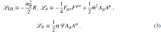
where, mP is the reduced Planck mass, R is the Ricci scalar, F
μv
≡ ∇
μ
A
v -
∇
v
A
μ
strength tensor associated to the vector field A
μ
with bare mass
 +
+
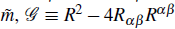
 is the Gauss-Bonnet topological invariant with coupling strength α whose dimensions are [α] = m-2
p, and R
μv
, R
μvρσ
are the Ricci tensor and the Riemann tensor, respectively. ℒ mf is the Lagrangian density for the energy content responsible for the inflationary period. The effective mass squared of the vector field is defined as
is the Gauss-Bonnet topological invariant with coupling strength α whose dimensions are [α] = m-2
p, and R
μv
, R
μvρσ
are the Ricci tensor and the Riemann tensor, respectively. ℒ mf is the Lagrangian density for the energy content responsible for the inflationary period. The effective mass squared of the vector field is defined as

Greek indices run from 0 to 3 and denote spacetime coordinates. Latin indices run from 1 to 3 and denote spatial components. In the case of the FLRW metric ds2 = dt2 - α 2 (t)dx2, where a(t) is the scale factor and x are the Cartesian spatial coordinates, the Gauss-Bonnet invariant reads

where H = ά/α is the Hubble parameter, and the overdot denotes a derivative with respect to the cosmic time t.
Perturbation spectrum
Having clarified our position with respect to the instability of the theory, we investigate the conditions for which the vector field obtains a nearly scale-invariant spectrum of superhorizon perturbations. The equation of motion for the vector field, which is obtained by varying the action of the Lagrangian in Eq. (2) with respect to A v , is

Assuming that inflation homogenizes the vector field; i.e. ∂ ¡ A μ = 0, it is easy to show that its temporal component, A t , must be zero, while the spatial components A i obey (See Appendix for the details of the calculations.)

Now, we perturb the vector field in the following way:

and write the equations of motion for transverse (δ
 ) and longitudinal (δ
 ) modes as follows (see Appendix ),
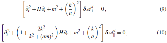
where δ
 are the Fourier modes of δAi . In the above equations, we used the fact that m2 is a constant during inflation since Ḣ ≃ 0 and therefore ℊ ≈ 24H4.
In order to quantize the field, we introduce creation/annihilation â†/ â operators for each polarization mode
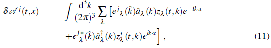
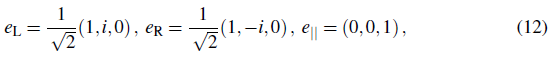
where λ = L, R labels the left and right transverse polarizations and λ = || the longitudinal polarization. Choosing the k-direction along the z-axis, the polarization vectors eλ can be written as
while the commutation rules are

With all the above, the power spectrum for the λ-polarized modes zλ is defined by
In the following subsections we study each polarization individually.
Transverse modes
Defining the physical transverse modes as b l, r ≡ z l,R/α and using the conformal time dη ≡ dt/α, the evolution equation (9) is rewritten as

with
 = αH being the Hubble parameter in conformal time. This equation can be recast in the form of a Bessel equation whose solution is given in terms of the Hankel functions H
v
as
= αH being the Hubble parameter in conformal time. This equation can be recast in the form of a Bessel equation whose solution is given in terms of the Hankel functions H
v
as

where

The constant C k can be found by matching Eq. (16) with the Bunch-Davies vacuum at early times (when -kη →∞) obtaining
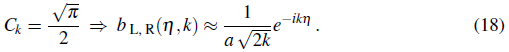
As expected, the modes behave as those for an oscillator. Now, we are interested in the late time behaviour (when -kη → 0) of the physical modes. In this regime, the dominant contribution of the solution in Eq. (16) is

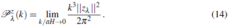
Replacing the later expression in the power spectrum defined in Eq. (14), we obtain
which corresponds to the scale dependance of the power spectrum of the physical vector field perturbations. The spectral index is written as
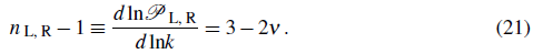
From Eqs. (17) and (21) it is clear that the physical vector field can attain a nearly flat power spectrum if and only if m2
≈-2H2. Consequently, the coupling α must satisfy
 + 24αH
4
2H2. Moreover, if
+ 24αH
4
2H2. Moreover, if
 « H, the condition for scale-invariance becomes
This result must be compared to the one in Refs. (Dimopoulos & Karciauskas, 2008; Himmetoglu et al., 2009a) where, instead of coupling the vector field to the Gauss-Bonnet invariant, the authors couple the vector field to the Ricci scalar, i.e. αRA μ A μ . In Refs. (Dimopoulos & Karciauskas, 2008; Himmetoglu et al., 2009a), it was shown that if the coupling constant is exactly 1/6 the power spectrum is perfectly flat, besides, the spectrum of each transverse mode is precisely the same as that for a scalar field. Finally, it is important to mention that the requirement m 2 ≈-2H 2 is precisely one of the possibilities discussed in (Karciauskas & Lyth, 2010) to avoid the instabilities mentioned in Sec. .
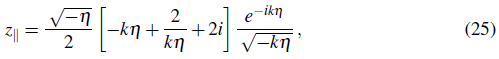
Longitudinal modes
Equation (10) gives the evolution for the longitudinal modes z∥, which, in terms of the conformal time, can be written as

Using the conditions
 = 0 and m
2 = - 2H
2 for a scale-invariant transverse power spectrum, and taking into account that the vacuum boundary condition is modified by
= 0 and m
2 = - 2H
2 for a scale-invariant transverse power spectrum, and taking into account that the vacuum boundary condition is modified by
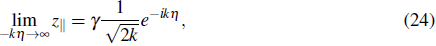
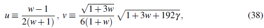
with ү =
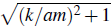 + 1 the Lorentz boost factor which takes us from the frame with k = 0 to the frame of momentum k ≠ 0, the solution of the above equation is (Dimopoulos et al., 2009, 2010.b, 2010.a; Dimopoulos, 2012)
which at late times (-kη→ 0) behaves as
 . Replacing the latter in the power spectrum in Eq. (14) we get
where we used the approximation H
2
≈, (αη)
-2
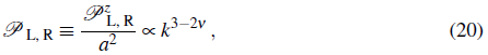
which is valid during inflation for a quasi-de Sitter background. As in the transverse case, the physical longitudinal power spectrum
 can be obtained by defining the physical longitudinal modes as b∥ ≡ z∥/α.
Statistical anisotropy
It is known that vector fields introduce inherently a preferred direction and therefore they can introduce large statistical anisotropies in the perturbation spectrum. If this is the case, the model will be ruled out because it is in disagreement with the observational results. For this reason, by using the 8N formalism (Starobinsky, 1985; Sasaki & Stewart, 1996; Lyth, Malik, & Sasaki, 2005; Lyth & Rodriguez, 2005.), in this section we compute the amount of statistical anisotropy in the spectrum, which is quantified in the parameter g defined in Eq. (1). We will show that g can be small enough to satisfy the observational bounds (Ade et al., 2016).
According to the δN formalism, the curvature perturbation ζ is the difference of the number of e-folds N between uniform density and spatially flat slices of spacetime: ζ ≡ δN. We will assume that N is function of the scalar field ф and the vector field: N = N(ф,A μ ).
Then, the curvature perturbation can be written as (Dimopoulos, 2012)
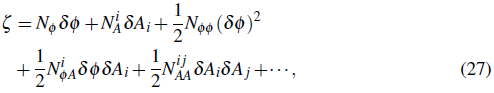
where
 and δA
i
are the perturbations of the scalar and vector field, respectively. From this result, the power spectrum of the curvature perturbation reads
and δA
i
are the perturbations of the scalar and vector field, respectively. From this result, the power spectrum of the curvature perturbation reads

where ,
 denotes the power spectrum of the scalar field, we have defined the even and odd polarizations for the transverse spectra as
 ± ≡
L
±
R
, respectively. We have taken into account that our theory is parity conserving, i.e.
R =
L, and thus
+ =
R
and
-
= 0. In the latter equation, we have also defined N
2
A
≡ llN
A
ll
2
≡ N
i
A
N
Ai
and
± ≡
L
±
R
, respectively. We have taken into account that our theory is parity conserving, i.e.
R =
L, and thus
+ =
R
and
-
= 0. In the latter equation, we have also defined N
2
A
≡ llN
A
ll
2
≡ N
i
A
N
Ai
and
 = N
A
/N
A
, which defines the preferred direction signaled by the vector field. By comparing the above equation with Eq. (1), we identify the isotropic part of the spectrum as
= N
A
/N
A
, which defines the preferred direction signaled by the vector field. By comparing the above equation with Eq. (1), we identify the isotropic part of the spectrum as

and hence the anisotropy parameter g can be written as
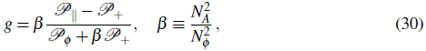
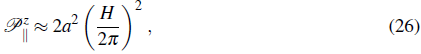
where β quantifies the relative contribution of the vector field over the scalar field to the modulation of N. Now, since the power spectra of the transverse solutions are nearly flat, they are given by
l,r ≈ (H/2π)2, and assuming that the potential of the scalar field is sufficiently flat during inflation, such that the power spectrum of the scalar field is also nearly flat at horizon exit (Lyth & Wands, 2002), i.e.
ф
≈ (H/2 π)2, we get
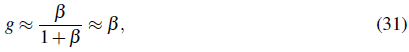
where we took into account that N is primarily modulated by the scalar field, since the vector field is subdominant during inflation, implying β «1, then g ≈ P « 1. This result agrees with the bounds given by Planck which suggest that g can be at most 0.97 (Ade et al., 2016).
Evolution of the vector field
In this section, we follow the evolution of the homogeneous vector field during and after inflation in order to determine if the vector field is able to play the role of a curvaton (Lyth & Wands, 2002; Dimopoulos, 2006).
Defining the physical components of the vector A i as B i ≡ A i /α and supposing, by simplicity, that B μ = (0,0,0, B), the equation of motion (7) is rewritten as

In the following, we solve this equation during and after inflation.
Evolution during inflation
As shown in section , the nearly scale-invariant spectrum of vector perturbations is obtained if the effective mass of the vector field is m 2 ≈-2H2, which remains constant during inflation because H ≃ constant. Therefore, the solution of Eq. (32) during inflation is

where B0 and B 1 are integration constants. The decaying mode in the solution in Eq. (33) is quickly diluted by inflation, thus the field is nearly constant given that B ≈ B0. This means that the vector field remains frozen and therefore it is not "erased" in the inflationary phase.
Evolution after inflation
The post-inflationary evolution of the vector field is also described by Eq. (32), but now H is time depending. Assuming that H evolves as
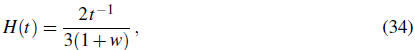
where w is the equation of state parameter of the dominant fluid after inflation and that αH 2 = ү, where ү is a constant (not necessarily the same required for a flat power spectrum), Eq. (32) can be recast in the following form

where
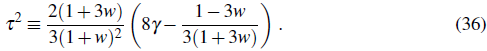
We assume this condition for simplicity, and having in mind the condition in Eq. (22) which is valid during inflation. The general solution of the above equation is

where
c 1 and c2 being constants of integration and J v and Y v being the Bessel functions of first and second kind, respectively. This solution should be contrasted with the solution for the equation of motion of a vector field non-minimally coupled to the Ricci scalar. In Ref. (Dimopoulos & Karciauskas, 2008), it was shown that, since this coupling is negligible after inflation if a radiation dominated period follows after the inflationary phase, since R ≈ 0 for an equation of state w ≈ 1/3, the vector field behaves as a massive minimally-coupled abelian vector. In contrast, in our model, the Gauss-Bonnet coupling contributes to the effective mass after inflation as well. This dependence is very important because, since the Gauss-Bonnet invariant changes its sign when passing from inflation to a matter or radiation dominated phase, naturally entails the change of sign of the vector mass. In Refs. (Dimopoulos, 2006; Dimopoulos & Karciauskas, 2008; Dimopoulos et al., 2010.b), it was shown that a vector field with positive mass after inflation can engage into quick oscillations, avoiding the generation of large-scale anisotropies. However, this sign change has to be assumed since a mechanism provoking this feature is not presented.
Now, we consider two possible approximations of the solution (37) regarding the dependence of the Bessel functions with respect to the bare mass m of the vector field. Firstly, we assume that the vector field is "light", i.e.
 t → 0. Hence the solution (37) is approximated by

where
 1
and
2 are constants. The latter solution means that the evolution of the light vector field is described by a power law for the scale factor. On the other hand, for a "heavy" vector field we take the limit of Eq. (37) when
t → ∞ obtaining
1
and
2 are constants. The latter solution means that the evolution of the light vector field is described by a power law for the scale factor. On the other hand, for a "heavy" vector field we take the limit of Eq. (37) when
t → ∞ obtaining

where b 1 and b 2 are constants. This solution shows that a heavy vector field oscillates with phase φ (which is a function of v) and envelope decreasing as

This shows that the vector field performs rapid oscillations, hence its dynamical behavior is effectively characterized by the envelope.
Evolution of the energy density
In the last section, we showed that the vector field has a constant magnitude during inflation. After inflation, it follows either a power law or an oscillatory motion depending whether it is light or heavy, respectively. However, if the vector field is to have a chance to imprint its perturbation spectrum at late times, it must nearly dominate the universe after inflation, according to the curvaton scenario (Lyth & Wands, 2002). Therefore, it is necessary to follow the evolution of its energy density.
Varying the corresponding action for the Lagrangian in Eq. (2) with respect to the metric g μv , it follows that (Carter & Neupane, 2006.; Nojiri, Odintsov, & Sasaki, 2005):
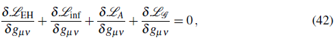
where
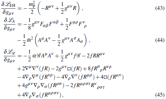
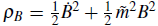
and f ≡ ½ αA μ . A μ Using the FLRW metric, the "00" component of Eq. (42) can be written as 3 m 2 p H 2 = ρinf + ρB, where ρinf is the energy density of the source driving inflation and
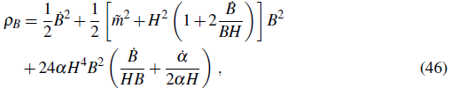
is the energy density of the physical vector field B
μ
= (0,0,0, B). This is to be compared with the energy density
 of a vector field non-minimally coupled to gravity through the Ricci scalar (Dimopoulos & Karciauskas, 2008; Karciauskas & Lyth, 2010; Golovnev et al., 2008.; Golovnev & Vanchurin, 2009; Golovnev, 2010). In our case, the energy density of the vector field has an extra term coming from the coupling with the Gauss-Bonnet invariant.
During inflation, Eq. (46) gives
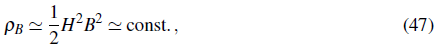
where we used the fact that
 « H and B, H and a are nearly constants. We can see that the energy density of the vector field is not diluted by inflation since it remains almost constant.
In order to avoid anisotropic expansion after inflation, the contribution to the energy tensor coming from the vector field must not introduce anisotropic pressures. This can be achieved if the vector field condensate behaves as a pressureless matter, i.e. p
B
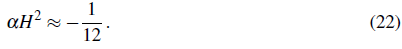
∝α-3 (Dimopoulos, 2006). In this section we investigate the available parameter space for the constant Y that allows this behavior in a radiation dominated universe characterized by w ≈ 1 /3. Before to continue our discussion, we want to point out the following. During inflation, the Gauss-Bonnet term is positive and it can be approximated by
 ≈ 24H4. On the other hand, in order to get a nearly flat power spectrum for the transverse modes we have αH
2
≈ - 1 /12, and therefore α < 0. After inflation, when the Hubble parameter H(t) is given by Eq. (34), the Gauss-Bonnet invariant is given by
≈ 24H4. On the other hand, in order to get a nearly flat power spectrum for the transverse modes we have αH
2
≈ - 1 /12, and therefore α < 0. After inflation, when the Hubble parameter H(t) is given by Eq. (34), the Gauss-Bonnet invariant is given by
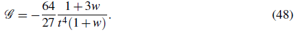
So, the Gauss-Bonnet invariant is negative if w > -1/3 (eg. a matter (w = 0) or a radiation (w = 1/3) fluid). This implies ү < 0 and a change in the sign of the effective mass, m2 =
 2 + α
2 + α
 , from negative, during inflation, to positive, after inflation. As explained in (Dimopoulos, 2006), a minimally-coupled vector plays the role of a curvaton if it has a negative mass-squared (explicitly m2
≈- 2H
2) during inflation. After inflation, the mass-squared has to become positive so that the vector field engages into oscillations and thus avoiding the production of large background anisotropy. As we show, in our model, this change of sign is tacitly provided by the "evolution" of the Gauss-Bonnet invariant.
, from negative, during inflation, to positive, after inflation. As explained in (Dimopoulos, 2006), a minimally-coupled vector plays the role of a curvaton if it has a negative mass-squared (explicitly m2
≈- 2H
2) during inflation. After inflation, the mass-squared has to become positive so that the vector field engages into oscillations and thus avoiding the production of large background anisotropy. As we show, in our model, this change of sign is tacitly provided by the "evolution" of the Gauss-Bonnet invariant.
Regarding a light field, we showed in Sec. that the dynamics of the vector field is described as a power law in the scale factor (see Eq. (39)). The power is given in terms of the equation of state parameter w and the constant Y. Then, replacing Eqs. (34) and (39) in Eq. (46), and considering that the dominant fluid after inflation can be either a stiff fluid (w = 1) or a radiation fluid (w = 1 /3), one can realize that is impossible to satisfy the condition that ү < 0 and the condition that the density of the vector field scales as pressureless matter, so we discard the light field solution.
For a heavy field, we showed that it is oscillating with decreasing envelope as α -3/2 . Following Ref. (Dimopoulos, 2006), the period of oscillations is much smaller than the Hubble time, which means that the effective behaviour of the vector field is given by its envelope. Therefore, replacing Eq. (41) in the density in Eq. (46) we get the average density over many oscillations as
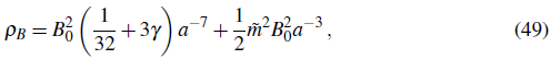
where B0 is the constant of proportionality implicit in Eq. (41). The first term in Eq. (49) goes as α -7 , so it decays faster than the radiation dominant fluid (which decays as α -4 ) and even faster than the second term. This means that p B ∝ α -3 . The fact that the average energy density decays as α -3 implies two important things: i) the vector field may eventually dominate the Universe and imprint its perturbation spectrum, and ii) the average energy density of the vector field scales as pressureless matter, so the average pressure is zero and therefore there is no generation of large background anisotropy.
Conclusions
In this paper, we have examined the evolution of a cosmological vector field coupled to the Gauss-Bonnet invariant. Assuming that
 « H, we found that, in order to get a nearly flat power spectrum for the transverse modes during inflation, the coupling a must satisfy the condition α H2 « -1/12. This implies that the power spectrum for the longitudinal modes is
 ll = 2
L
R
. Consequently, we showed that the amount of statistical anisotropy in our model, quantified by the parameter g, is within the observational bounds, given that the vector field is subdominant during inflation. We also found that the vector field remains constant during the inflationary phase, but it performs rapid oscillations after that whenever
» H. Averaging over many oscillations, the vector field effectively decays as α
-3/2
, which means that the average energy density, pB, decays as α
-3
, so, after inflation, the vector field behaves like a pressureless fluid. This indicates that the vector field has a chance to nearly dominate the universe after inflation, without introducing large background anisotropy, and thus be able to imprint its curvature perturbation.
ll = 2
L
R
. Consequently, we showed that the amount of statistical anisotropy in our model, quantified by the parameter g, is within the observational bounds, given that the vector field is subdominant during inflation. We also found that the vector field remains constant during the inflationary phase, but it performs rapid oscillations after that whenever
» H. Averaging over many oscillations, the vector field effectively decays as α
-3/2
, which means that the average energy density, pB, decays as α
-3
, so, after inflation, the vector field behaves like a pressureless fluid. This indicates that the vector field has a chance to nearly dominate the universe after inflation, without introducing large background anisotropy, and thus be able to imprint its curvature perturbation.
According to the vector curvaton scenario, the mass of the vector must be negative during inflation and positive after that. In our model, this feature is provided by the particular behavior of the Gauss-Bonnet invariant because it changes its sign when passing from inflation to a matter or radiation dominated epoch. Therefore, we conclude that this non-minimal coupling between a vector field and the Gauss-Bonnet invariant can be a reliable and realistic vector curvaton model.

