


 English (pdf)
 Article in xml format
 Article references
 Send this article by e-mail
 Cited by SciELO
  Cited by Google
  Similars in
SciELO
Similars in
SciELO  Similars in Google
 Permalink
Introduction
Throughout human history, several pandemics have significantly reduced world population (Hays, 2005; Huremović, 2019). For instance, a century ago the world was afflicted by the Spanish flu epidemic (H1N1), which began and peaked in 1918 and persisted until 1920 (Hays, 2005; Huremović, 2019). This pandemic was one of the first in which data and statistics (from 48 countries) allowed health authorities to estimate that 40.1 million people died, i.e., 2.1% of the world's population at that time (Barro, et al., 2020). On the other hand, the COVID-19 coronavirus disease (SARS-Cov-2) pandemic is the first with data available in real-time (Dong, et al., 2020) on the time series of the total confirmed cases, confirmed cases per day, total deaths, deaths per day, active cases, total test results, etc., for each country (Worldometers, 2021). The availability of time series for confirmed cases and deaths (GitHub, 2021) from January 1, 2020, to September 15, 2021, allowed us to detect some properties also found in a wide variety of complex systems.
Recently, different aspects of the spread of the COVID-19 pandemic have been studied from the point of view of complex systems (Holovatch, et al., 2017). Just to mention a few of these studies, researchers analyzed the spatial evolution of the Covid-19 pandemic around the world based on the coronavirus cases time series per country using a particular type of neural network called self-organizing maps to show that it has behaved similarly in certain groups of countries (Melin, et al., 2020). In another study, time series of daily infections per country were analyzed using a methodology developed to study network problems showing that there are groups of countries with differentiated contagion dynamics (Álvarez, et al., 2020). Moreover, by using a toy model for social networks and the so-called small-world network, researchers explained why most COVID-19 infection curves are linear (Thurner, et al., 2020). On the other hand, three clusters of countries and territories with similar profiles of standardized COVID-19 time dynamics were identified by using a machine learning technique (António, et al., 2021). Besides, times series of active and cumulative cases from three countries were analyzed in the context of a continuous effective model based on a modified diffusion equation under Lifshitz scaling to describe some aspects of the SARS-Cov-2 virus diffusion and to reproduce the spreading of the pandemic between two cities of Brazil (Anacleto, et al., 2020). Additionally, based on confirmed cases in the US distributed across more than 2,000 counties, researchers found that the right tail of this distribution exhibited a power law with Pareto exponent close to one (Beare & Toda, 2020). Furthermore, the formalism of the propagation of a wave packet in a dispersive medium was used to describe the spreading of the COVID-19 pandemic in Italy (Feoli, et al., 2020). Finally, a mathematical framework was developed to study the economic impact of pandemics like the COVID-19 by integrating epidemiological dynamics with a kinetic model of wealth exchange (Dimarco, et al., 2020).
As a result of the first stage into a research program in progress about the spreading of the COVID-19 pandemic based on the analysis of empiric data from January 2020 to September 2021, it is evident that the COVID-19 pandemic has spread around the world exhibiting complex system properties such as lognormal laws, temporal fluctuation scaling, and time correlation. In contrast with Beare & Toda's results (2020), where the cumulative confirmed cases distributed among the US counties exhibited a power law, in the present study, the daily cumulative numbers of confirmed cases and deaths distributed among the countries of the world exhibited lognormal laws. In this respect, it should be mentioned that lognormal laws emerge in a wide variety of complex systems in different science fields (Limpert, et al., 1991) because of the presence of stochastic multiplicative processes in them (Mitzenmacher, 2004). It is also clear in this paper that temporal fluctuation scaling (TFS) behaves as a power-law relation between the standard deviation and the mean when these are calculated for the daily cumulative number of confirmed cases and deaths distributed among countries in the world. With respect to this property, from a general perspective, fluctuation scaling affirms the existence of a power-law relation between the standard deviation and the mean of a time series (Eisler & Kertész, 2006; Eisler, et al., 2008; Fronczac & Fronczac, 2010). Fluctuation scaling can be seen in two different forms (Eisler, et al., 2008): The ensemble fluctuation scaling and the TFS (Eisler & Kertész, 2006; Fronczac & Fronczac, 2010). Since the discovery of the fluctuation scaling by Smith (1938) and Taylor (1961), this property has been found in complex systems in areas such as social science, life science, ecology, economics, financial markets, climatology, city traffic, complex networks, physics, etc. (Eisler, et al., 2008; Fronczac & Fronczac, 2010). On the other hand, temporal fluctuation scaling has also been observed in the daily return time series of cases and deaths per day in the world, but this time following the Lévy alpha-stable distribution. The time correlation for these daily return time series has been detected by calculating the Hurst exponents. Regarding this property, it is important to mention that time correlation means that the autocovariance function decays exponentially by a spectral that tends to infinity (Stanley, 1971; Mantegna & Stanley, 2000; Grau-Carles, 2000) in such a way that, at the critical point, the said exponential decay turns into a power-law decay (Varotsos, et al., 2002). It should be emphasized that time series associated with different types of complex systems exhibit time correlations as evidenced in nucleotide sequences, neuron activity, cardiac interbeat intervals, earthquake processes, variation of daily maximum temperatures, literary texts, stock index variations, electric signals, etc. (Martín-Montoya, et al., 2015). It is important to insist that time correlation is detected by calculating the Hurst exponent (Martín-Montoya, et al., 2015), a property also detectable if the time series is not large enough (Sánchez-Granero, et al., 2008; Trinidad-Segovia, et al., 2012). Power-law correlations in time can be measured by a scaling parameter or fractal dimension, but if the time series is self-similar, this fractal dimension is related to the Hurst exponent (Feder, 1994; Chen, et al., 2008).
The present study showed that the daily cumulative number of confirmed cases and deaths in world countries from March 31, 2020 to September 15, 2021 followed lognormal distributions with two parameters using a similar methodology to that developed to fit the gamma probability density function to wealth distributions obtained in the context of a non-conservative kinetic model of wealth exchange with production saving (Quevedo & Quimbay, 2020). As for the daily cumulative numbers of confirmed cases and deaths among world countries for a given period, it was evident that the standard deviations and the means were related as power laws, which implies the existence of TFS in the system using an analogous procedure to that presented by Abril & Quimbay (2021) to show that the TFS and the temporal evolution of its exponent in some financial time series can be described by using the path-integral formalism.
In the second part of the paper, the same procedure was used to show that the TFS is also observed in the daily return time series of cases and deaths per day, but this time with a Lévy stable distribution. For these daily return time series, which are not large enough, the existence of time correlation was detected by calculating the Hurts exponents using a modification of the classical R/S method as in Martín-Montoya, et al. (2015) in their calculation of the Hurst exponents for seismic time series in Colombia given that they were not large enough.
It is important to emphasize that at this stage, the present study does not aspire to explain why the complex system properties identified emerged, as that is the objective of later phases of the research program. In the future, then, the hope is to formulate stochastic models aimed at explaining from a microscopic perspective the emergence of those properties. It is also relevant to mention that the second stage of the aforementioned research program will aim at showing how the properties identified in the spread of COVID-19 in the world also express themselves at the country level, or that such properties exist inside countries when the spread is considered at this level.
Data related to the COVID-19 pandemic spreading in the world
The starting point of this work is the data from confirmed cases and deaths by COVID-19 available in GitHub (2021). Thus, the cumulative number of confirmed cases per country has been organized daily starting on January 1, 2020, with 27 confirmed cases in China and ending on September 15, 2021, with 226.477.919 confirmed cases in 193 countries and 721 confirmed cases in an international zone. The cumulative number of deaths per country were also organized daily, starting on January 11, 2020, with one death in China and ending on September 15, 2021, with 4.666.083 deaths in 186 countries and 15 deaths in the international zone. On the other hand, the number of new confirmed cases per day was also daily organized per country starting on January 2, 2020, with no confirmed new cases in China and ending on September 15, 2021, with 563.272 confirmed cases in 160 countries. Finally, the number of new deaths was daily organized per country starting on January 12, 2020, with no confirmed new deaths in China and ending on March 15, 2021, with 10.358 new deaths in 132 countries.
Figure 1 shows that the increase in the number of countries with confirmed cases of COVID-19 (curve in blue color) was large for the period between January 1, 2020, and March 31, 2020, increasing from 1 to 180 (179 countries and 1 international zone) while it was much smaller between April 1, 2020, and September 15, 2021, from 180 to 194. Likewise, the number of countries with deaths by COVID-19 (curve in orange color) passed from one on January 11, 2020, to 127 on March 30, 2020 (126 countries and 1 international zone) while it increased from 130 on April 1, 2020, to 187 on September 15, 2021. Figure 1 also shows a similar behavior for both curves except for a threshold of an approximate average of 18 days: the blue curve grew from 32 on February 22, 2020, to 148 on March 17, 2020, while the orange curve grew from 27 on March 10, 2020, to 147 on April 7, 2020.
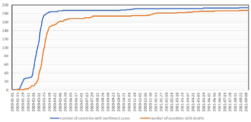
As shown in figure 1, the spread of the COVID-19 pandemic had a vertiginous progress in the world as the number of countries with confirmed cases and deaths grew strongly from January 1, 2020 to March 30, 2020. During this period, the daily evolution of the number of countries had an analogous behavior to the time evolution of the entropy in the case of a close economical system when states are out of equilibrium (Drăgulescu & Yakovenko, 2000). The economic system described with the kinetic model of money exchange by Drăgulescu & Yakovenko (1990) reaches the Boltzmann-Gibbs distribution of money only when the entropy is at a maximum and the system is in equilibrium. It has been proven that from January 1, 2020 to March 30, 2020 the daily distributions of cumulative numbers of confirmed cases and deaths among world countries do not fit by using any of the probability density functions. Moreover, in the next section it will be evident that only after March 30, 2020 these daily distributions were very well fitted to lognormals.
Temporal fluctuation scaling
The daily cumulative numbers of confirmed cases and deaths in the world distributed among countries fitted by lognormal distributions with two parameters of the form
where o is the shape parameter and |r the location parameter. The goodness of fit was checked in all the cases by the following significance tests: Kolmogorov-Smirnov, Anderson-Darling, and Chi-square. In all cases, the goodness of fit was very good from March 31, 2020 on. According to the significance tests, it should be noted that these fits to lognormal distributions were not completely valid for the period before March 31, 2020 possibly because before this day the system was in a non-equilibrium state as suggested by the results in figure 1.
Table 1 presents the results of the fit parameters to lognormal distributions of two parameters for daily cumulative numbers of confirmed cases and deaths in the world by taking their distributions among the countries and shows the values of the fit parameters to lognormal distributions o and |r for 36 days. As already mentioned, for all cases, the goodness of the fit was very good. The daily values of the mean (M) and the standard deviation (SD) are also shown in the Table.
Table1. Fit parameters to lognormal distributions for 36 days, and means and standard deviations for the cumulative numbers of confirmed cases and deaths
| Day | Cumulative number of confirmed cases | Cumulative number of deaths | ||||||
|---|---|---|---|---|---|---|---|---|
| σ | μ | M | SD | σ | μ | M | SD | |
| 31/03/2019 | 2.916 | 5.087 | 4868 | 20116 | 2.242 | 2.546 | 352 | 1490 |
| 15/04/2020 | 2.670 | 6.167 | 11318 | 53948 | 2.447 | 3.357 | 949 | 4068 |
| 30/04/2020 | 2.672 | 6.741 | 17729 | 85711 | 2.563 | 3.802 | 1516 | 6656 |
| 15/05/2020 | 2.655 | 7.169 | 24331 | 114147 | 2.556 | 4.148 | 1966 | 8604 |
| 31/05/2020 | 2.618 | 7.597 | 33096 | 14493 | 2.575 | 4.362 | 2327 | 9983 |
| 15/06/2020 | 2.634 | 7.900 | 43011 | 177739 | 2.566 | 4.645 | 2739 | 11211 |
| 30/06/2020 | 2.600 | 8.199 | 55930 | 231135 | 2.525 | 4.922 | 3191 | 12443 |
| 15/07/2020 | 2.610 | 8.452 | 72558 | 309640 | 2.535 | 5.097 | 3613 | 13800 |
| 31/07/2020 | 2.597 | 8.705 | 94140 | 412085 | 2.572 | 5.239 | 4093 | 15582 |
| 15/08/2020 | 2.576 | 8.926 | 114871 | 504236 | 2.527 | 5.445 | 4629 | 17498 |
| 31/08/2020 | 2.576 | 9.108 | 136402 | 595951 | 2.483 | 5.618 | 5147 | 19348 |
| 15/09/2020 | 2.588 | 9.259 | 158270 | 690979 | 2.480 | 5.749 | 5649 | 21009 |
| 30/09/2020 | 2.609 | 9.407 | 181879 | 791157 | 2.459 | 5.876 | 6117 | 22595 |
| 15/10/2020 | 2.692 | 9.523 | 207270 | 885885 | 2.465 | 5.989 | 6608 | 24078 |
| 31/10/2020 | 2.782 | 9.685 | 24415 | 994757 | 2.466 | 6.130 | 7177 | 25604 |
| 15/11/2020 | 2.910 | 9.802 | 287600 | 1139732 | 2.508 | 6.248 | 7852 | 27196 |
| 30/11/2020 | 2.979 | 9.908 | 33205 | 1315768 | 2.597 | 6.356 | 8715 | 29353 |
| 15/12/2021 | 3.006 | 10.041 | 385597 | 1538143 | 2.552 | 6.508 | 9683 | 32338 |
| 31/12/2020 | 3.007 | 10.172 | 437894 | 1768852 | 2.614 | 6.567 | 10625 | 35620 |
| 015/01/2021 | 2.984 | 10.313 | 492266 | 2019684 | 2.752 | 6.547 | 11461 | 39042 |
| 31/01/2021 | 3.058 | 10.376 | 536884 | 221070 | 2.725 | 6.679 | 12701 | 43321 |
| 15/02/2021 | 3.036 | 10.465 | 56916 | 2331830 | 2.694 | 6.780 | 13700 | 46832 |
| 28/02/2021 | 3.029 | 10.532 | 594961 | 241284 | 2.681 | 6.847 | 14419 | 49338 |
| 15/03/2021 | 3.000 | 10.616 | 626440 | 2501671 | 2.701 | 6.883 | 15081 | 51656 |
| 31/03/2021 | 2.995 | 10.709 | 671621 | 2621873 | 2.654 | 6.978 | 15989 | 54412 |
| 15/04/2021 | 3.000 | 10.789 | 724650 | 2775073 | 2.672 | 7.024 | 16874 | 57130 |
| 30/04/2021 | 2.971 | 10.880 | 788838 | 3003525 | 2.704 | 7.064 | 17872 | 60020 |
| 15/05/2021 | 2.965 | 10.946 | 846772 | 3261210 | 2.720 | 7.101 | 18831 | 63026 |
| 31/05/2021 | 3.029 | 10.965 | 884902 | 3437211 | 2.689 | 7.183 | 19827 | 66280 |
| 15/06/2021 | 3.010 | 11.025 | 915537 | 3539547 | 2.679 | 7.244 | 20685 | 69229 |
| 30/06/2021 | 2.999 | 11.084 | 944355 | 3614917 | 2.691 | 7.275 | 21242 | 71121 |
| 15/07/2021 | 2.997 | 11.150 | 979219 | 3686200 | 2.666 | 7.346 | 21887 | 72777 |
| 31/07/2021 | 2.994 | 11.229 | 1025572 | 3793871 | 2.656 | 7.433 | 22692 | 74432 |
| 15/08/2021 | 2.976 | 11.308 | 1074355 | 3926953 | 2.630 | 7.503 | 23453 | 75964 |
| 31/08/2021 | 3.044 | 11.338 | 1122840 | 4090524 | 2.631 | 7.542 | 24173 | 77801 |
| 15/09/2021 | 3.009 | 11.412 | 1167411 | 4244528 | 2.563 | 7.622 | 24920 | 79817 |
This system presents TFS because SD and M are related as a power law of the form
where C is a factor and D is the TFS exponent. Using the SD and M values in table 1, for the 15 data from the period between March 31, 2020 and October 31, 2020, the fit parameters to the power law for cumulative numbers of confirmed cases were C=5.2073 and D=0.9839, with a coefficient of determination R2=0.9981, while for the cumulative number of deaths they were C=7.0154 and D=0.9281 with R2=0.9984. Additionally, for the 9 data from the period between November 15, 2020 and March 15, 2021, the fit parameter to power law for the cumulative numbers of confirmed cases were C=2.4953 and D=1.0369 with ii!2=0.9973, while these parameters for the cumulative numbers of deaths were C=3.0786 and D=1.0107 with R2=0.9984. Finally, for the 12 data from the period between March 31, 2021 to September 15, 2021, the fit parameter to power law for the cumulative numbers of confirmed cases were C=21.556 and D=0.8732 with R2=0.9905, while for the cumulative numbers of deaths they were C=11.667 and D=0.8733 with R2=0.9951. It can be seen that for the first period (March 31, 2020-October 31, 2020), the TFS exponents were less than one for both cases, for the second period (November 15, 2020-March 15, 2021) they were greater than one, and for the third period (March 31, 2021-September 15, 2021) they were less than one.
Astonishingly, this system presents another temporal property, but in this case, the location parameter |i of the fit to a lognormal distribution and the mean (M) are related also as a power law of the form
where E is a factor and F is the exponent. For the first period (March 31, 2020- October 31, 2020), the fit parameters to the power law for the cumulative numbers of confirmed cases were E=1.4442 and F=0.1561 with R2=0,9782 while for the cumulative numbers of deaths they were E=0.4382 and F=0.2979 with R2=0,9982. For the second period (November 15, 2020-March 15, 2021), the fit parameters to the power law for the cumulative numbers of confirmed cases were E=2.7213 and F=0.1017 with R2=0.9917, while for the cumulative numbers of deaths they were E=1.7543 and F=0.1419 with R2=0.9755. For the third period (March 31, 2021-September 15, 2021), the fit parameter to the power law for the cumulative numbers of confirmed cases were E=2.2306 and F=0.1167 with R2=0.9823, while for the cumulative numbers of deaths they were E=0.8404 and F=0.2172 with R2=0.9713.
For periods of half a month (T), the standard deviations (SD) and the means (M) calculated daily both for the cumulative numbers of confirmed cases and deaths in the world (cumulative numbers that are distributed among the countries) were related as power laws of the form
where C(T) is the factor depending on the period T and D(T) is the TFS exponent depending on T. This power law relation means that for periods of half a month this system also presented TFS. The fit parameters to the power law are presented in table 2; it is evident that the R 2 in all the cases is remarkably close to 1 indicating an excellent fit to a power law in all the cases. For the case of cumulative numbers of confirmed cases, the smallest TFS exponent (D-cases) was 0.5344 for the period July-I-21 while the largest was 1.1704 for the period May-I-21. On the other hand, in the case of cumulative numbers of deaths, the smallest TFS exponent (D-deaths) was 0.6192 for the period July-II-21 while the larger was 1.1943 for the period January-I-21.
Table 2 Power-law fit parameters C and D, and R2 associated with the TFS of the cumulative numbers of confirmed cases and deaths for periods of half a month
| Period | Cumulative # of confirmed cases | Cumulative # of deaths | ||||
|---|---|---|---|---|---|---|
| C | D | R 2 | C | D | R2 | |
| April-I-20 | 1.316 | 1.1396 | 0.9956 | 3.390 | 1.0338 | 0.9999 |
| April-II-20 | 3.469 | 1.0340 | 0.9998 | 2.819 | 1.0598 | 0.9994 |
| May-I-20 | 18.163 | 0.8660 | 0.9998 | 5.793 | 0.9630 | 0.9987 |
| May-II-20 | 48.645 | 0.7687 | 0.9999 | 12.733 | 0.8598 | 0.9993 |
| June-I-20 | 39.896 | 0.7875 | 0.9998 | 40.246 | 0.7114 | 0.9994 |
| June-II-20 | 3.129 | 1.0252 | 0.9992 | 47.871 | 0.6892 | 0.9996 |
| July-I-20 | 0.959 | 1.1333 | 0.9998 | 12.790 | 0.8524 | 0.9955 |
| July-II-20 | 1.497 | 1.0937 | 0.9999 | 5.459 | 0.9558 | 0.9927 |
| August-I-20 | 3.573 | 1.0176 | 1 | 5.886 | 0.9475 | 0.9994 |
| August-II-20 | 5.446 | 0.9814 | 0.9999 | 5.234 | 0.9614 | 0.9996 |
| September-I-20 | 5.194 | 0.9855 | 0.9999 | 14.360 | 0.8434 | 0.9939 |
| September-II-20 | 6.638 | 0.9651 | 0.9998 | 8.345 | 0.9065 | 0.9995 |
| October-I-20 | 26.273 | 0.8517 | 0.9996 | 14.649 | 0.8419 | 0.9995 |
| October-II-20 | 117.040 | 0.6960 | 0.9998 | 35.966 | 0.7398 | 0.9991 |
| November-I-20 | 22.808 | 0.8606 | 0.9978 | 65.053 | 0.6729 | 0.9991 |
| November-II-20 | 4.133 | 0.9967 | 0.9995 | 34.273 | 0.7444 | 0.9997 |
| December-I-20 | 3.168 | 1.0178 | 0.997 | 6.563 | 0.9264 | 0.9996 |
| December-II-20 | 1.226 | 1.0918 | 0.9998 | 2.479 | 1.0324 | 0.9982 |
| January-I-21 | 0.899 | 1.1159 | 0.9998 | 0.554 | 1.1943 | 0.9956 |
| January-II-21 | 2.664 | 1.0330 | 0.9988 | 2.869 | 1.0183 | 0.9996 |
| February-I-21 | 14.757 | 0.9033 | 0.9996 | 2.245 | 1.0443 | 0.9996 |
| February-II-21 | 83.190 | 0.7728 | 0.9999 | 2.398 | 1.0372 | 0.9997 |
| March-I-21 | 261.680 | 0.6867 | 0.9997 | 2.302 | 1.0414 | 0.9957 |
| March-II-21 | 285.310 | 0.6801 | 0.9998 | 11.268 | 0.8763 | 0.9992 |
| April-I-21 | 98.633 | 0.7592 | 0.9996 | 7.759 | 0.9149 | 0.9941 |
| April-II-21 | 6.985 | 0.9552 | 0.9986 | 13.542 | 0.8576 | 0.9979 |
| May-I-21 | 0.376 | 1.1704 | 0.9999 | 5.319 | 0.9529 | 0.9980 |
| May-II-21 | 0.769 | 1.1183 | 0.993 | 3.346 | 0.9999 | 0.9996 |
| June-I-21 | 33.975 | 0.8417 | 0.999 | 2.450 | 1.0314 | 0.9990 |
| June-II-21 | 409.060 | 0.6605 | 0.9979 | 7.695 | 0.9165 | 0.9898 |
| July-I-21 | 2318.300 | 0.5344 | 0.9994 | 37.612 | 0.7573 | 0.9993 |
| July-II-21 | 570.170 | 0.6360 | 0.9984 | 149.440 | 0.6192 | 0.9993 |
| August-I-21 | 86.507 | 0.7722 | 0.9989 | 125.610 | 0.6365 | 0.9991 |
| August-II-21 | 9.326 | 0.9325 | 0.9982 | 21.157 | 0.8135 | 0.9973 |
| September-I-21 | 7.332 | 0.9498 | 0.9981 | 18.661 | 0.8259 | 0.9961 |
Figure 2 shows the time evolution of the TFS exponents for cumulative numbers of confirmed cases (D-cases) and those of deaths (D-deaths) from the values in table 2: TFS exponents for cumulative numbers of confirmed cases (curve in blue color) had five peaks in the periods April-I-20, July-I-20, January-I-21, May-I-21, and September-I-21 and those for cumulative numbers of deaths (curve in orange color) also had five peaks but in the periods April-II-20, August-II-20, January-I-21, June-I-21, and September-I. It should be noted that these peaks were associated with the COVID-19 pandemic peaks registered until now considering the time series of confirmed cases per day and deaths per day in the world (GitHub, 2021). Based on these time series, the following procedure was applied to each of the time series: (i) The average of the data for 20 consecutive days served to construct the average time series; (ii) then, these were normalized with respect to their maximum value (normalized average time series), and finally, (iii) attention was focused on these normalized average times series for cases per day and deaths per day. For the cases per day, it was evident that the peaks were on April 13, 2020, July 30, 2020, January 8, 2021, May 6, 2021, and September 1, 2021, while for deaths per day, the peaks were on April 24, 2020, August 16, 2020, January 29, 2021, May 9, 2021, and September 3, 2021.
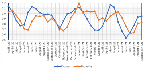
Figure 2 Time evolution of TFS exponents for the cumulative numbers of confirmed cases and deaths in periods of a-half month
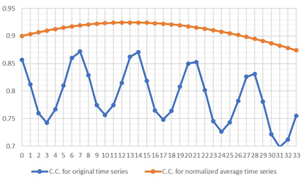
The correlation coefficient between the TFS exponents represented in the two curves in figure 2 is 0.421. If it is assumed that the orange curve has a one-period lag with respect to the blue curve, then the correlation coefficient is 0.727, which suggests that the behavior of confirmed cases per day would be reflected approximately 15 days after in the behavior of the deaths per day and, therefore, the existence of a 14-day lag between the times series of confirmed cases per day and the deaths per day may be confirmed. To do so, the correlation coefficients are calculated as a function of the lag in the number of days for the original time series of confirmed cases per day and deaths per day (curve in blue color in figure 3), and for the normalized average time series of confirmed cases per day and deaths per day (curve in orange color in figure 3). In figure 3 the correlation coefficient shows a maximum value in both cases with a 14-day lag so the maximum value for the time series of confirmed cases per day is 0.871 while that for the normalized average time series of confirmed cases per day is 0.924. It is clear that the correlation coefficients calculated for the time series of confirmed cases per day and deaths per day exhibit an oscillating behavior with a 7-day period.
Time correlation
Considering the time series of confirmed cases per day and deaths per day in the world (GitHub, 2021), the daily return times series of confirmed cases per day CD(t) and deaths per day DD(t) were constructed by defining the daily return of confirmed cases per day (DRCD) in the following form: DRCD(t+1) = [CD(t+1)-CD(t)]/CD(t); similarly, the daily return of deaths per day (DRDD) was expressed as DRDD(t+1)=[DD(t+1)-DD(t)]/DD(t). These definitions implied that the daily return represented the percentage change of the respective quantity between two successive days: t + 1 and t. In the next step, January 22, 2020, was defined for both daily return time series as the first date and September 15, 2021, as the last date, each with a total of 603 data. Starting from these daily return time series, time subseries having different numbers of data were constructed for each case so that for all the time subseries, the first data was on January 22, 2020. The number of data of the first daily return time subseries was 60, corresponding to the period from January 22, 2020, to March 21, 2020. The second daily return time subseries had 75 data, corresponding to the period from January 22, 2020, to April 5, 2020, which meant that the increase in the number of data between two consecutive time subseries was 15. Thus, the third time subseries had 90 data, corresponding to the period between January 20, 2020 and April 20, 2020. Taking the possible increments of 15 data, the total number of time subseries that could be constructed was 37. For instance, the time subseries number 36 had 585 data corresponding to the period from January 22, 2020 to October 28, 2021, and the last one had 603 data corresponding to the period from January 16, 2020 to September 15, 2021, which matched the original daily return time series.
For each one of the time subseries of confirmed cases per day and deaths per day, the following quantities were calculated: (i) mean; (ii) standard deviation; (iii) the four fit parameters to a Lévy distribution notated as α, β, μ, and σ, and (iv) the Hurst exponent (H) calculated by using a modification of the classical R/S method as in Martín-Montoya, et al. (2015). The results of these calculations are presented in table 3.
Table 3 Results of the calculation of the mean, the standard deviation, the fit parameters to a Lévy distribution, and the Hurst exponent for each one of the time subseries of confirmed cases per day and deaths per day defined by each period.
| Daily return time subseries of confirmed cases per day | |||||||||
|---|---|---|---|---|---|---|---|---|---|
| Per. | From | Until | St. Dev. | Mean | alpha | beta | mu | sigma | Hurst |
| 1 | 2020-01-22 | 2020-03-21 | 0.7844 | 4.5739 | 1.1321 | 0.2129 | 0.3166 | 0.2441 | 0.4852 |
| 2 | 2020-01-22 | 2020-04-05 | 0.6407 | 4.0949 | 0.9976 | 0.0200 | -0.8735 | 0.1848 | 0.4751 |
| 3 | 2020-01-22 | 2020-04-20 | 0.5383 | 3.7421 | 0.9984 | 0.0074 | -0.4302 | 0.1716 | 0.5140 |
| 4 | 2020-01-22 | 2020-05-05 | 0.4622 | 3.4668 | 0.9877 | 0.1635 | -1.1301 | 0.1383 | 0.5301 |
| 5 | 2020-01-22 | 2020-05-20 | 0.4070 | 3.2445 | 0.9881 | 0.1569 | -0.9681 | 0.1201 | 0.5280 |
| 6 | 2020-01-22 | 2020-06-04 | 0.3644 | 3.0601 | 0.9897 | 0.1768 | -1.0067 | 0.1142 | 0.4646 |
| 7 | 2020-01-22 | 2020-06-19 | 0.3308 | 2.9040 | 1.1476 | 0.2250 | 0.1345 | 0.1122 | 0.4995 |
| 8 | 2020-01-22 | 2020-07-04 | 0.3018 | 2.7698 | 1.1799 | 0.2608 | 0.1194 | 0.1008 | 0.5004 |
| 9 | 2020-01-22 | 2020-07-19 | 0.2776 | 2.6526 | 1.1919 | 0.3038 | 0.1167 | 0.1029 | 0.4939 |
| 10 | 2020-01-22 | 2020-08-03 | 0.2565 | 2.5492 | 1.2257 | 0.3271 | 0.1015 | 0.1006 | 0.4981 |
| 11 | 2020-01-22 | 2020-08-18 | 0.2397 | 2.4570 | 1.2566 | 0.3347 | 0.0899 | 0.0993 | 0.5204 |
| 12 | 2020-01-22 | 2020-09-02 | 0.2246 | 2.3741 | 1.2734 | 0.2974 | 0.0762 | 0.0966 | 0.5299 |
| 13 | 2020-01-22 | 2020-09-17 | 0.2113 | 2.2992 | 1.3115 | 0.2782 | 0.0643 | 0.0957 | 0.5406 |
| 14 | 2020-01-22 | 2020-10-02 | 0.1990 | 2.2309 | 1.3354 | 0.3201 | 0.0626 | 0.0946 | 0.5608 |
| 15 | 2020-01-22 | 2020-10-17 | 0.1892 | 2.1684 | 1.3561 | 0.2684 | 0.0537 | 0.0934 | 0.5491 |
| 16 | 2020-01-22 | 2020-11-01 | 0.1805 | 2.1109 | 1.3774 | 0.2665 | 0.0507 | 0.0936 | 0.5934 |
| 17 | 2020-01-22 | 2020-11-16 | 0.1723 | 2.0578 | 1.4029 | 0.2607 | 0.0473 | 0.0936 | 0.5838 |
| 18 | 2020-01-22 | 2020-12-01 | 0.1650 | 2.0085 | 1.4349 | 0.2553 | 0.0439 | 0.0939 | 0.5992 |
| 19 | 2020-01-22 | 2020-12-16 | 0.1603 | 1.9638 | 1.4204 | 0.2504 | 0.0441 | 0.0942 | 0.6073 |
| 20 | 2020-01-22 | 2020-12-31 | 0.1540 | 1.9210 | 1.4319 | 0.2413 | 0.0421 | 0.0943 | 0.6129 |
| 21 | 2020-01-22 | 2021-01-15 | 0.1480 | 1.8809 | 1.4396 | 0.2144 | 0.0388 | 0.0939 | 0.6012 |
| 22 | 2020-01-22 | 2021-01-30 | 0.1413 | 1.8433 | 1.4791 | 0.2213 | 0.0359 | 0.0943 | 0.5890 |
| 23 | 2020-01-22 | 2021-02-14 | 0.1351 | 1.8080 | 1.4791 | 0.1909 | 0.0319 | 0.0957 | 0.6152 |
| 24 | 2020-01-22 | 2021-03-01 | 0.1305 | 1.7745 | 1.4927 | 0.2259 | 0.0326 | 0.0959 | 0.6164 |
| 25 | 2020-01-22 | 2021-03-16 | 0.1275 | 1.7429 | 1.4926 | 0.2795 | 0.0358 | 0.0963 | 0.6139 |
| 26 | 2020-01-22 | 2021-03-31 | 0.1243 | 1.7128 | 1.5092 | 0.3072 | 0.0368 | 0.0967 | 0.6347 |
| 27 | 2020-01-22 | 2021-04-15 | 0.1209 | 1.6842 | 1.5251 | 0.3422 | 0.0374 | 0.0971 | 0.6392 |
| 28 | 2020-01-22 | 2021-04-30 | 0.1173 | 1.6570 | 1.5272 | 0.3611 | 0.0374 | 0.0958 | 0.6296 |
| 29 | 2020-01-22 | 2021-05-15 | 0.1131 | 1.6311 | 1.5331 | 0.3806 | 0.0364 | 0.0949 | 0.6174 |
| 30 | 2020-01-22 | 2021-05-30 | 0.1104 | 1.6075 | 1.5185 | 0.3739 | 0.0358 | 0.0949 | 0.6424 |
| 31 | 2020-01-22 | 2021-06-14 | 0.1069 | 1.5839 | 1.5297 | 0.3837 | 0.0344 | 0.0946 | 0.6391 |
| 32 | 2020-01-22 | 2021-06-29 | 0.1045 | 1.5613 | 1.5419 | 0.4019 | 0.0346 | 0.0947 | 0.6192 |
| 33 | 2020-01-22 | 2021-07-14 | 0.1024 | 1.5396 | 1.5567 | 0.4021 | 0.0341 | 0.0948 | 0.6258 |
| 34 | 2020-01-22 | 2021-07-29 | 0.1003 | 1.5188 | 1.5662 | 0.3648 | 0.0322 | 0.0949 | 0.6482 |
| 35 | 2020-01-22 | 2021-08-13 | 0.0986 | 1.4991 | 1.5692 | 0.3242 | 0.0309 | 0.0957 | 0.6613 |
| 36 | 2020-01-22 | 2021-08-28 | 0.0961 | 1.4803 | 1.5572 | 0.3001 | 0.0296 | 0.0964 | 0.6639 |
| 37 | 2020-01-22 | 2021-09-15 | 0.0943 | 1.4589 | 1.5441 | 0.3296 | 0.0306 | 0.0975 | 0.6665 |
| Daily return time subseries of deaths per day | |||||||||
| Per. | From | Until | St. Dev. | Mean | alpha | beta | mu | sigma | Hurst |
| 1 | 2020-01-22 | 2020-03-21 | 2.4080 | 9.4464 | 1.0129 | 0.3799 | 5.1485 | 0.2737 | 0.5286 |
| 2 | 2020-01-22 | 2020-04-05 | 1.9430 | 8.4868 | 0.9007 | 0.2479 | -0.2688 | 0.2039 | 0.5480 |
| 3 | 2020-01-22 | 2020-04-20 | 1.6233 | 7.7723 | 0.9705 | 0.3077 | -1.2154 | 0.1884 | 0.6107 |
| 4 | 2020-01-22 | 2020-05-05 | 1.3944 | 7.2124 | 1.0336 | 0.3261 | 1.1189 | 0.1774 | 0.6132 |
| 5 | 2020-01-22 | 2020-05-20 | 1.2208 | 6.7586 | 1.0781 | 0.3865 | 0.5342 | 0.1676 | 0.6294 |
| 6 | 2020-01-22 | 2020-06-04 | 1.0951 | 6.3816 | 1.1013 | 0.3929 | 0.4097 | 0.1667 | 0.6530 |
| 7 | 2020-01-22 | 2020-06-19 | 0.9896 | 6.0608 | 1.1223 | 0.4774 | 0.3849 | 0.1613 | 0.6554 |
| 8 | 2020-01-22 | 2020-07-04 | 0.8995 | 5.7843 | 1.1468 | 0.4709 | 0.2962 | 0.1549 | 0.6862 |
| 9 | 2020-01-22 | 2020-07-19 | 0.8262 | 5.5423 | 1.1638 | 0.4976 | 0.2635 | 0.1493 | 0.6973 |
| 10 | 2020-01-22 | 2020-08-03 | 0.7643 | 5.3285 | 1.1875 | 0.5079 | 0.2247 | 0.1468 | 0.6876 |
| 11 | 2020-01-22 | 2020-08-18 | 0.7129 | 5.1374 | 1.1885 | 0.5284 | 0.2216 | 0.1413 | 0.6916 |
| 12 | 2020-01-22 | 2020-09-02 | 0.6659 | 4.9658 | 1.1917 | 0.5353 | 0.2084 | 0.1362 | 0.7016 |
| 13 | 2020-01-22 | 2020-09-17 | 0.6273 | 4.8108 | 1.1867 | 0.5467 | 0.2129 | 0.1347 | 0.6966 |
| 14 | 2020-01-22 | 2020-10-02 | 0.5919 | 4.6691 | 1.2051 | 0.5222 | 0.1846 | 0.1361 | 0.6883 |
| 15 | 2020-01-22 | 2020-10-17 | 0.5607 | 4.5393 | 1.2216 | 0.5446 | 0.1722 | 0.1348 | 0.6987 |
| 16 | 2020-01-22 | 2020-11-01 | 0.5323 | 4.4197 | 1.2489 | 0.5673 | 0.1577 | 0.1371 | 0.7130 |
| 17 | 2020-01-22 | 2020-11-16 | 0.5083 | 4.3090 | 1.2772 | 0.6053 | 0.1499 | 0.1389 | 0.7325 |
| 18 | 2020-01-22 | 2020-12-01 | 0.4868 | 4.2062 | 1.2891 | 0.6343 | 0.1489 | 0.1389 | 0.7418 |
| 19 | 2020-01-22 | 2020-12-16 | 0.4659 | 4.1106 | 1.3058 | 0.6426 | 0.1394 | 0.1386 | 0.7540 |
| 20 | 2020-01-22 | 2020-12-31 | 0.4467 | 4.0213 | 1.3102 | 0.6601 | 0.1379 | 0.1379 | 0.7568 |
| 21 | 2020-01-22 | 2021-01-15 | 0.4297 | 3.9376 | 1.3139 | 0.6676 | 0.1359 | 0.1378 | 0.7641 |
| 22 | 2020-01-22 | 2021-01-30 | 0.4136 | 3.8591 | 1.3181 | 0.6662 | 0.1315 | 0.1375 | 0.7710 |
| 23 | 2020-01-22 | 2021-02-14 | 0.3977 | 3.7853 | 1.3347 | 0.6659 | 0.1236 | 0.1406 | 0.7692 |
| 24 | 2020-01-22 | 2021-03-01 | 0.3845 | 3.7153 | 1.3486 | 0.6809 | 0.1199 | 0.1415 | 0.7736 |
| 25 | 2020-01-22 | 2021-03-16 | 0.3725 | 3.6491 | 1.3637 | 0.6953 | 0.1168 | 0.1428 | 0.7767 |
| 26 | 2020-01-22 | 2021-03-31 | 0.3607 | 3.5862 | 1.3746 | 0.6993 | 0.1123 | 0.1421 | 0.7854 |
| 27 | 2020-01-22 | 2021-04-15 | 0.3496 | 3.5265 | 1.3769 | 0.7042 | 0.1105 | 0.1412 | 0.7837 |
| 28 | 2020-01-22 | 2021-04-30 | 0.33877 | 3.4697 | 1.3861 | 0.7049 | 0.1056 | 0.1399 | 0.7776 |
| 29 | 2020-01-22 | 2021-05-15 | 0.32817 | 3.4155 | 1.3929 | 0.7013 | 0.1003 | 0.1379 | 0.7862 |
| 30 | 2020-01-22 | 2021-05-30 | 0.31784 | 3.3639 | 1.3895 | 0.7039 | 0.0985 | 0.1357 | 0.8142 |
| 31 | 2020-01-22 | 2021-06-14 | 0.30939 | 3.3147 | 1.3882 | 0.7251 | 0.1001 | 0.1357 | 0.8183 |
| 32 | 2020-01-22 | 2021-06-29 | 0.30098 | 3.2674 | 1.3919 | 0.7295 | 0.0986 | 0.1345 | 0.8158 |
| 33 | 2020-01-22 | 2021-07-14 | 0.29289 | 3.222 | 1.4 | 0.7211 | 0.0932 | 0.1327 | 0.8337 |
| 34 | 2020-01-22 | 2021-07-29 | 0.28764 | 3.1794 | 1.3953 | 0.6972 | 0.0917 | 0.1323 | 0.8338 |
| 35 | 2020-01-22 | 2021-08-13 | 0.28034 | 3.1377 | 1.3978 | 0.7004 | 0.0899 | 0.1311 | 0.8402 |
| 36 | 2020-01-22 | 2021-08-28 | 0.2731 | 3.0975 | 1.3994 | 0.7052 | 0.0883 | 0.1299 | 0.832 |
| 37 | 2020-01-22 | 2021-09-15 | 0.26617 | 3.0514 | 1.4038 | 0.7149 | 0.0884 | 0.1305 | 0.8348 |
The existence of another type of TFS is apparent given that SD(t) and M(t) are related as a power law of the form
where K is a factor and L is the TFS exponent. Using the values of SD(t) and M(t) shown in table 3, the fit parameters to the power law for daily returns of confirmed cases per day were K=5.2595 and L=0.5372, with R2=0.9997, while these parameters for daily returns of deaths per day were K=6.0527 and L=0.5159, with R2=0.9997.
Astonishingly, this system had another TFS because the standard deviation of the daily returns of deaths per day SDDRD(t) and the mean of the daily returns of confirmed cases per day DMRCC(t) were related as a power law of the form
where P is a factor and Q is the TFS exponent. Using the values of SDDRD(t) and MDRCC(t) in table 3, the following fit parameters to this power law were obtained: P=10.905 and Q=0.5225, with R2=0.9994. The reason for this result is that SDDRD(t) and the standard deviation of daily returns of confirmed cases per day SDDRCC(t) had a linear relation of the form SDDRED(t) = 2.062* SDDRCC(t) + 0.0581, with R2=0.9999. This implies that the correlation coefficient between the standard deviations SDDRED(t) and SDDRCC(t) in table 3 should be 1 and, effectively, this correlation coefficient was 0.9999718. This result implies that the behavior of the daily returns of deaths per day was highly correlated to the behavior of the daily returns of confirmed cases per day as validated by the fact that the mean of the daily returns of deaths per day MDRD(t) was related with the mean of the daily returns of confirmed cases MDRCC(t) through the linear relation MDRD(t) =3.074* MDRCC(t) - 0.0226, with R2 =0.9999.
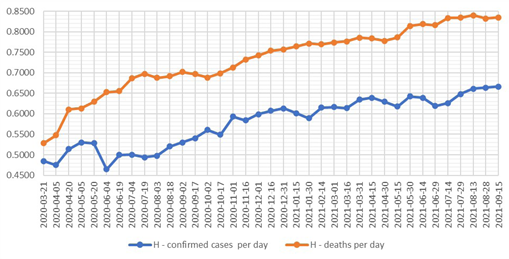
On the other hand, the Hurts exponents of the daily returns of confirmed cases per day and those of the daily returns of deaths per day in table 3 are represented in figure 4 where the evolution on time for the Hurts exponents of the daily returns of confirmed cases per day (blue color curve) and for those of the daily returns of deaths per day (orange color curve) are shown. The time correlation behavior as anti-persistent (H<0,5) was detected for the daily returns of confirmed cases per day in the following periods: January 22, 2020, to March 21, 2020; January 22, 2020, to April 5, 2020; January 22, 2020, to June 4, 2020; January 22, 2020, to June 19, 2020; January 22, 2020, to July 19, 2020, and January 22, 2020, to August 3, 2020. The behavior of the time correlation was persistent (H>0,5) for the other 31 periods. This persistent behavior grew continuously on time as the Hurst exponent for the period between January 22, 2020, and August 18, 2020, was 0.5204 while between January 22, 2020, and September 15, 2021, it was 0.6665. Additionally, the behavior of the short-long correlation in time was persistent (H>0,5) only for the daily returns of deaths per day for the 37 periods, a behavior that grew continuously with time as the Hurst exponent for the period from January 22, 2020, to March 31, 2020 was 0.5286 and from January 22, 2020 to September 15, 2021 it was 0.8348.
Conclusions
The availability of the time series of confirmed cases and deaths (GitHub, 2021) from January 1, 2020, to September 15, 2021, allowed for the detection of complex system properties such as lognormal laws, temporal fluctuation scaling, and time correlation in the spreading of the COVID-19 pandemic around the world.
During the period from January 1, 2020, to March 31, 2020, the spread of the COVID-19 pandemic had vertiginous progress in the world as the number of countries with confirmed cases and deaths increased. Besides, during the period from January 1, 2020, to March 30, 2020, the daily distributions of cumulative numbers of confirmed cases and deaths among countries did not fit any probability density function because the system behaved as if it were in a non-equilibrium state. Consequently, only after March 30, 2020, these daily distributions perfectly fitted lognormals of two parameters as the system behaved in an equilibrium state.
For periods of half a month, the standard deviations and the means calculated daily both for the cumulative numbers of confirmed cases and for those of deaths in the world were related as power laws as a manifestation of the TFS. Specifically, the values of the TFS exponents depended on the period considered and their values were between 0.53 and 1.19. Moreover, the TFS exponents for cumulative numbers of confirmed cases showed five peaks in the periods April-I-20, July-I-20, January-I-21, May-I-21, and September-I-21 and the TFS exponents for cumulative numbers of deaths also had five peaks but in the periods April-II-20, August-II-20, January-I-21, June-I-21, and September-I and they were associated with the five peaks that the COVID-19 pandemic around the world had had until September 15, 2021.
Starting from the daily return times series of confirmed cases and deaths per day and taking all the possible increments of 15 data between two successive time subseries for each case, the total number of daily returns time subseries constructed was 37. For all these daily return time subseries, the mean, the standard deviation, the fit parameters to a Lévy distribution and the Hurst exponent were calculated. It should be mentioned that the Hurst exponents were calculated by using a modification of the classical R/S method used when the time series is not large enough. The standard deviations and the means of all the daily returns time subseries for confirmed cases and deaths per day were related as power laws indicating the existence of another type of TFS in the system. Also, the standard deviations of the daily returns of deaths and the means of those of confirmed cases per day were related as a power law meaning that the daily returns of deaths per day were highly correlated to those of confirmed cases per day.
The presence of complex system properties in the spreading of the COVID-19 pandemic at world level was determined by considering the world as constituted by countries, although they were also found when smaller regions were considered. In another study in progress, it has been shown that these properties are also present at country level considering countries as constituted by states and, similarly, they are present as well at state level when it is assumed these are constituted by counties indicating that the properties identified here are invariant when the spatial scale changes.
These results are consistent with the stochastic nature of the spread of the COVID-19 pandemic around the world. Consequently, a stochastic model aimed at explaining it should lead to the emergence of the complex system properties identified in this paper.

