


 Inglés (pdf)
 Articulo en XML
 Referencias del artículo
 Enviar articulo por email
 Citado por SciELO
  Citado por Google
  Similares en
SciELO
Similares en
SciELO  Similares en Google
 Permalink
Introduction
The term interference refers to peculiar spatial characteristics of the distribution of light energy propagating in free space or the quantum particles moving in field-free regions. In such environments, light waves and single massive (non-relativistic) particles, respectively, obey the classical wave equation and the Schrödinger equation (Born & Wolf, 1993; Mandel & Wolf, 1995; Feynman et al., 1965; Feynman & Hibbs, 1965). However, it is well known that interference is exhaustively described by the spatial (or time-independent) components of these equations regardless of the differences between their time propagators.
The Helmholtz equation describes the spatial components of both the classical wave equation in free space and the Schrödinger equation for field-free regions. The classical or quantum context for the Helmholtz equation is specified by its eigenvalue, i.e., it involves the wave frequency in the case of light but the momentum in the case of massive particles. This mathematical generality of interference implies that its phenomenology (i.e., its description in ordinary space, which is the environment of the corresponding experiments) in any classical and quantum contexts should be supported by a unique principle.
Although wave superposition is widely accepted as a fundamental principle of physics, in the case of interference with massive particles, it does not refer to ordinary space but to a mathematical environment called Hilbert space (Feynman et al., 1965). As a consequence, in quantum interference, the wave superposition cannot provide a phenomenological description but only a predictive estimation of the experimental outcomes. The prediction accuracy of the interference patterns with massive particles, strongly supported by the experimental outcomes (Matteucci, 2011; Bach etal., 2013; Tavabi etal., 2019), cannot hide the lack of phenomenological generality of the wave superposition.
An alternative notion, i.e., the confinement in spatially-structured Lorentzian wells, overcomes this limitation of wave superposition by maintaining the mathematical accuracy of the classical and quantum interference predictions. Indeed, this notion leads to the description of interference with waves and single massive particles in ordinary space. Its mathematical and physical features have been discussed in detail (Castañeda & Matteucci, 2017; Castañeda et al., 2021) and illustrated with predictions of experimental patterns obtained specifically with single electrons and molecules (Castañeda et al., 2016a, 2016b; Castañeda & Matteucci, 2017). For this reason, the confinement in spatially-structured Lorentzian wells has been proposed as the unique general principle of interference (Castañeda et al., 2021).
A conceptual discussion of confinement phenomenology is pertinent and necessary to clearly appreciate its differences and advantages as compared with the standard optical and quantum formalisms. In this paper, the confinement ability of space is discussed and special attention is paying to its spatial structuration. It has been shown that nonlocality prepared on a mask triggers the build-up of interference patterns (Castañeda & Matteucci, 2019). Subsequently, the geometric nature of the prepared nonlocality is contrasted with the standard notion that conceives it as a physical property of waves or particle beams moving in the setup, and a very special feature of the spatially structured confinement under strong nonlocality, called spatial entanglement, is discussed. Such a feature ensures disjoint distributions of the confinement zones whose cross-sections account for the highly contrasted interference patterns. A summary of the analysis and the conclusions is then presented at the end of the paper.
For an appropriate analysis, symbolic mathematics and illustrations are used while the discussions are focused on the meaning of the expressions rather than on their algebraic definitions and developments, which are not included here but can be revisited in several previous papers (Castañeda & Matteucci, 2017, 2019; Castañeda et al., 2016a, 2016b, 2021).
¿Can free-space confine?
In the standard interference formalisms, free space is a Newtonian concept, i.e., a uniform, isotropic, and passive scenario where physical phenomena take place. Accordingly, interference features are completely attributed to the properties of waves and particles, which leads to a phenomenological description of wave interference in ordinary space but only as far as the prediction of single-particle interference in the Hilbert space is concerned.
Nevertheless, it has been shown that a general phenomenological description of interference in ordinary space both with waves and single particles can be accurately formulated by regarding free space from a non-Newtonian perspective, i.e., as a physical system with a geometrical behavior (Castañeda & Matteucci, 2017, 2019; Castañeda et al., 2021). To analyze it, let us start by considering the configuration of a non-paraxial interference setup as conceptually depicted in figure 1. In the preparation and measurement (P&M) scheme, it is realized by three planes (labeled S, M, and D) that delimit two consecutive stages in the setup, i.e., the preparation (SM) stage between S and M separated by a distance Z, and the measurement (MD) stage between M and D at a distance z from each other. The reduced coordinates (r′A r′D) and (ξ A , ξ D ) (Castañeda et al., 2020) are defined at the S and M planes, respectively, to determine univocally pairs of points on them, which are denoted as r′± = r′A ± r′D /2 and ξ± = ξ A ± ξ D /2, while individual points at the D plane are determined by the coordinate rA.
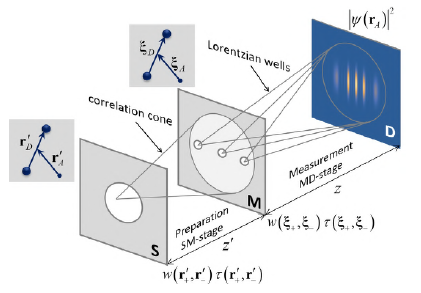
Figure 1 Conceptual sketch of the interference setup in the P&M scheme. S: source plane, M: mask plane, and D: detector plane. The reduced coordinates at the S and M planes are indicated, A correlation cone is depicted in the preparation SM stage, and individual spatially-structured Lorentzian wells are depicted in the measurement MD stage. The mathematical expressions are explained in the text.
The spatial components of both the classical wave equation in free space and the Schrodinger equation for field-free regions are given by the Helmholtz equation ∇2ψ + k
2ψ = 0 where ψ is the eigenfunction of the Laplacian operator at any point in the setup, with eigenvalue -k
2
, and k =ω/c for frequency waves ω and k = p
The exact solution of the Helmholtz equation for any point in the setup can be obtained by applying Green’s theorem (Arfken, 1970), which leads to the eigenfunction at the D plane in terms of the expansion (Castañeda et al., 2020)

where Θ(ξ A , r A , z, k) denotes Green’s functions defined in the volume of the MD stage, a set of orthogonal, geometrical, time-independent, deterministic, and complex valued eigenfunctions of the Laplacian operator. Indeed, Green’s functions connect each ξ A point on the M plane with any r A point on the D plane, as pointed out by their arguments. The explicit mathematical form of Θ(ξ A , r A , z, k) is deduced in Castañeda & Matteucci (2019).
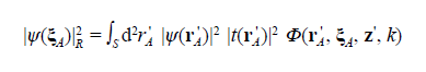
The aim of the setup in figure 1 is to measure the spatial distribution of the optical field irradiance or the single particle arrivals at the D plane by attaching a square modulus detector there. Such measurements are proportional to the physical observable
 , so Eq. (1) allows expressing it straightforwardly in terms of the expansion:

over the geometric, deterministic, time-independent, and complex-valued kernel

defined in the volume of the MD stage. In Eq. (2), it is worth noting that the measurement of the physical observable at the D plane explicitly implies the requirement of nonlocality prepared as a boundary condition at the M plane, which is formalized by the product of the non-locality function (Castañeda et al., 2021).

and the non-local transmission function (Castañeda et al., 2021)

The term “nonlocal(ity)” refers to the dependence on pairs of points (ξ+, ξ-) in the ordinary space of the functions defined in Eqs. (3) to (5). Additionally, these functions have Hermitic symmetry related to the permutation of such points, i.e., Φ(ξ+, ξ-, r, z, k) = Φ* (ξ-, ξ+, r, z, k), w(ξ+, ξ-) = w* (ξ-, ξ+), and τ(ξ+, ξ-) = τ* (ξ-, ξ+). They also include local components determined for ξ+ = ξ- = ξA, i.e. ξD = 0, which take respectively the forms Φ(ξ A , r A , z, k) = |Θ(ξ A , r A , z, k)|2, i.e., real-valued and positive definite local-kernel modes, w(ξ A , ξ A ) = |ψ(ξ A )|2, the physical observable that describes the spatial distribution of the light irradiance or the quantum probability of single particle arrivals at the M plane, and τ(ξ A , ξ A ) = |t(ξ A )|2 with 0 ≤ |t(ξ A )|2 ≤ 1, the transmittance placed at the M plane.
For the phenomenology, it is crucial to separate the local and non-local contributions from the M plane in Eq. (2). It is straightforwardly performed by manipulating the integration limits appropriately, thus expressing the physical observable at the D plane as
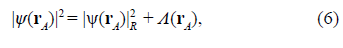
with

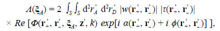
a real-valued and positive-definite function, i.e., a physical observable defined at the D plane, and
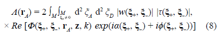
with Re denoting the real part, which is obtained by considering the Hermitic symmetry of the integrand and by adding the contributions due to the two degrees of freedom in the orientation of the separation vectors realized by the permutation of the pair of points, i.e., ξ
D
↔ -ξ
D
. The real-valued function Λ (rA) in Eq. (8) takes on positive and negative values to achieve
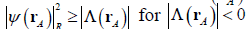 .
.
It is important to discuss at this point some features of the expressions above. The nonlocality function differs from the two-point spatial correlation (called in optics the cross-spectral density) (Born & Wolf, 1993) in that the first does not involve the ensemble average over a great enough number of experimental realizations that the second does. The nonlocality function denotes a single component of the ensemble corresponding to an individual experimental realization. This term refers to the event that begins with a local emission of a wave disturbance or a single particle at the S plane and ends with its local detection at the D plane. Consequently, Eq. (2) describes the detection of a local and instantaneous value of light energy or the arrival of a single particle to the detector.
This formalization of the individual experimental realizations is not explicitly considered in the standard interference formalisms. In optics, the light is regarded as a stochastic process (Mandel & Wolf, 1995) and the detector averages its energy fluctuations during the integration time. Such time average equals the ensemble average because of the ergodicity of light (Mandel & Wolf, 1995). The ensemble average of Eq. (2) leads to the conventional description of the cross-spectral density propagation (Mandel & Wolf, 1995). However, the current technology is capable of single photon detection, so Eq. (2) has become experimentally feasible in optics with no need for averaging.
In quantum mechanics, a single particle moves randomly in field-free regions of ordinary space while Eq. (2) is regarded as the prediction calculation of the experimental outcomes in the Hilbert space. From this point of view, Eq. (2) cannot account for the phenomenological description of the single particle behavior in the setup. Furthermore, the ensemble average of Eq. (2) is required because the predicted interference pattern is built up after recording a great enough number of random individual particle arrivals to the detector.
As shown in the next section, the stochastic fluctuations of light, as well as the random appearance of the interference build-up with single particles, are closely related to the emission properties of the source. However, the preparation of the non-locality function w(ξ+, ξ-) is profoundly geometric and related to the SM stage configuration. This feature, together with the geometric definition of the non-local kernel Φ(ξ+, ξ-, r, z, k), related to the MD stage configuration, suggests that Eq. (2) can actually describe the phenomenology of individual experimental realizations of interference with light and single particles in ordinary space.
Interference is a conservative phenomenon. Consequently, the conservation law of the light energy, as well as the normalization of the quantum probabilities at the M and D planes, lead to the condition

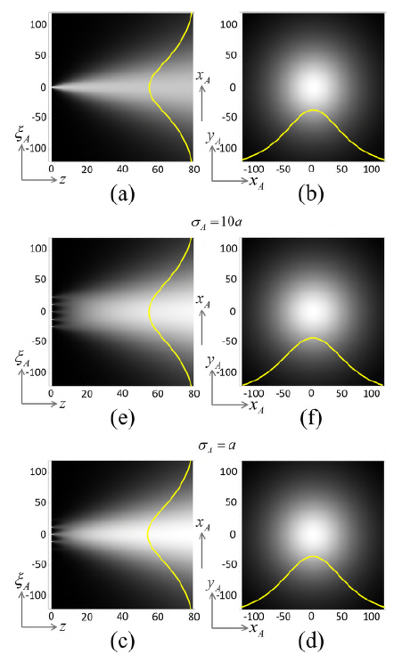
Figure 2 Axial sections for 0 ≤ z ≤ 20λ (where λ = 4 pm is the de Broglie wavelength for single matter particles and λ = 4pm is the wavelength for light waves) on the left column and cross-sections at z = 20 λ on the right column of |ψ(rA)| 2 R for a mask whose transmission function has a linear regular array of five point-openings with a spacing of α = 3 λ at the M plane (left extreme of the axial sections). A Gaussian boundary condition |ψ(ξ A )|2 ∝ exp[-|ξA|2/(2σ A 2 )] is established at this plane with variable standard deviation whose values ensure the isolation of the central opening in (a) and (b), the inclusion of three openings in (c) and (d), and the covering of the complete array in (e) and (f). The axes units are pm for single matter particles and for light waves.
The replacement of Eqs. (6) to (8) in (9) leads straightforwardly to

and ∫ D d2 r A Λ(r A ) = 0,, which implies

at any distance z ≥ 0 from the M plane.
To discuss the phenomenological meaning and implications of these results, let us look at the graphs |ψ(r A )| R 2 in figure 2 and Λ (r A ) in figure 3 for specific but representative examples. According to the specifications in the figure 2 caption, the boundary condition (a Gaussian light irradiance distribution or a Gaussian quantum probability at the M plane) determines the number of array openings at which the light disturbance or a single particle can enter the MD stage depending on the value of the standard deviation σa. In (a), (b), it isolates the central opening at ξ A = 0, thus reducing Eq. (7) to |ψ(r A )| R 2 = |ψ(0)|2 |t(0)|2 Φ(0, r A , z, k) and Eq. (8) to null. Consequently, the observable recorded by the detector is |ψ(r A )|2 = |ψ(r A )|R 2 .. The same result is obtained by blocking all the openings around the central one. It seems, then, that two or more openings should remain open and be crossed by light disturbances or single particles to obtain non-null values for Eq. (8), although only one opening is crossed in each individual realization.
The kernel mode Φ(0, r A , z, k) describes the cone in the MD stage with the vertex at ξA = 0 (Figure 2a), and rotation symmetric cross-section with Lorentzian profile at any distance z from the vertex (Figure 2b). The boundary condition |ψ(0)|2 |t(0)|2 denotes the local value of the light energy or the quantum probability of the single particle that emerges from the mask at the cone vertex. The physical observable |ψ(r A )| R 2 i.e., the cross-section of the cone at the D plane, denotes the spatial distribution of the light energy, as well as the quantum probability over the detection area. The normalization in Eq. (10) indicates that: (i) the light energy entering the cone at its vertex will distribute completely in the cone cross-section at any distance from the vertex, or (ii) the single particle that crosses the mask at the cone vertex will move to the D plane within the cone. In other words, the light energy, as well as the single particle, will be confined in the cone volume, so that the cone is actually a well. The Lorentzian cross-section of the well indicates that the light energy concentrates or the single particle moves preferably around the well axis.
In figure 2c-d, σ A grows to cover three openings of the mask placed at ξ A = -a, 0, a so the Lorentzian wells Φ(ξ A , r A , z, k),, with vertices at these three points, appear in the volume of the MD stage. If the nonlocality function at the mask plane nullifies, then the physical observable at the D plane is described by
This means that the light disturbances or the single particles at the vertex of each well, represented by the boundary condition |ψ(ξ A )|2 |t(ξ A )|2,, will be confined only within the respective well even if the wells overlap. It should be highlighted that the cross-section of the complete well at a long enough distance from the mask plane in the overlapping region becomes Lorentzian too.
Because of the independent confinements, the set of individual Lorentzian wells is separable. This means that the physical observable ψ(r A )|R 2 R at a given point r A on the D plane results by adding the values of the light energy or the single particles confined in each individual well arriving to r A , as expressed by Eq. (7). Furthermore, the total light energy or single particles recorded by the detector must equal the energies of the light disturbances or the single particles confined in each individual Lorentzian well (i.e., those that cross their vertices), as expressed by Eq. (9).
This analysis is confirmed by the graphs in figure 2e-f, where σ A is wide enough to cover the complete array, and individual Lorentzian wells with vertices at ξ A = -2a, -a, 0, a, 2a should be considered.
Summarizing, the component |ψ(r A )| R 2 of the physical observable |ψ(r A )|2 is also a physical observable at the D plane that allows characterizing the propagation of the light disturbances and the single particles in the MD stage in terms of their confinement in individual Lorentzian wells. These wells are mathematically formalized by the kernel modes Φ(ξ A , r A , z, k), independently from the nature (wave or particle) of the confined physical entity, so that all the Lorentzian wells have the same geometry.
This suggests that the Lorentzian wells are a fundamental geometric behavior of space that is related to the propagation of waves in free space and to single massive particles in field-free regions, which can be observed by measuring the physical observable |ψ(r A )| R 2 . The measurement is feasible by completely removing the prepared nonlocality. This observable is the local component of |ψ(r A )|2 in the sense that it relates the wave disturb-ance or the single particle that crosses the mask only at the vertex of the Lorentzian well with its local detection at any point of the well cross-section at the D plane.
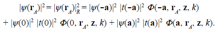
It should be emphasized that the Lorentzian wells cannot mutually modulate spatially, as illustrated in figure 2c-f, which means that the overlapping of wells with vertices at different mask openings is not a condition for interference. To produce the interference modulation, the term A(r A ) must be added to |ψ(r A )| R 2, as expressed in Eq. (6). This relates the nonlocality prepared at the boundary of the MD-stage: w(ξ +, ξ -) τ(ξ +, ξ -) with the local detection of light energy or single particles at any point of the well cross-section. In this sense, Λ(r A ) denotes the non-local component of |ψ(r A )|2 . More precisely, the prepared nonlocality triggers the spatial oscillations of Λ(r A ) in the volume of the MD stage according to the geometry of the non-local kernel Φ(ξ +, ξ -, r A , z, k) in Eq. (8), as illustrated in figure 3.
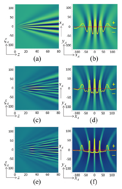
Figure 3 Axial sections for ≤ z ≤ 20λ (λ = 4pm for single matter particles and 4pm for light waves) on the left column and cross-sections at z = 20 λ on the right column of Λ (r A ) for linear regular arrays of (a), (b) two, (c), (d) three, and (e), (f) five point-openings with a spacing of α = 3 λ at the M plane (left extreme of the axial sections) under the boundary condition w(ξ +, ξ -) τ(ξ +, ξ -) = 1. The axes units are pm for single matter particles and pm for light waves.
Therefore, the prepared nonlocality is the necessary and sufficient condition for interference because it causes the spatial modulation of the individual Lorentzian wells, thus determining specific distributions of confinement zones in their volumes oriented in space by the non-local phase α(ξ +, ξ -) + ϕ(ξ +, ξ -) (Castañeda & Matteucci, 2017, 2019, Castañeda et al., 2021). Consequently, the light energy and the single particles will be concentrated in such confinement zones, so that the interference pattern is observed at the cross-section on the D plane of the complete spatially-structured Lorentzian well as it is illustrated in figure 4.
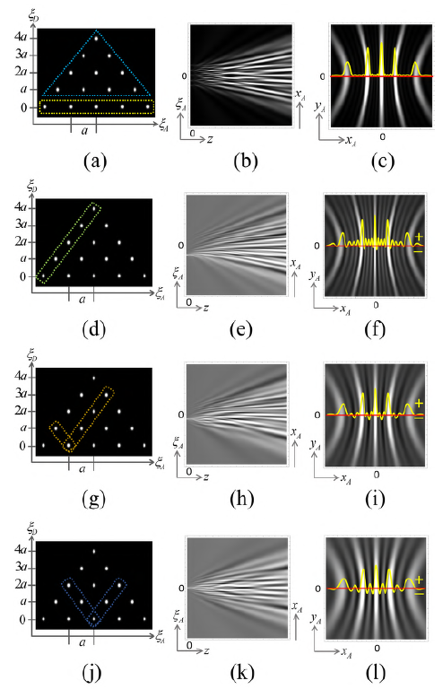
Figure 4 The spectrum of classes of point emitters on the left column for the Lorentzian wells in Figure 2(e), (f) and the geometric potential in Fig. 3 (e), (f). Axial and cross-sections (at z = 103 λ) of spatially-structured Lorentzian wells on the middle and right columns. In (a) the dotted line rectangle for ξ D = 0 encloses the vertices of the individual Lorentzian wells for a mask with a linear array of point openings with a spacing of α = 3λ while the triangle encloses the vertices of the 10 geometric potential modes (ξ D ≠ 0) under strong nonlocality covering all the mask openings. Graphs (b) and (c) describe the complete well resulting from the overlapping of the five individual spatiallystructured wells, three of them, with vertices at ξ A = -2a, -a, 0, are depicted in graphs (d)-(l). The rectangles in the spectra of classes of point emitters in (d), (g), and (j) show the specific subset of four geometric potential modes that modulate the individual Lorentzian well whose vertex is enclosed in the rectangles. Consequently, the resulting individual spatially-structured Lorentzian wells in (e)-(l) exhibit different modulations.
Nevertheless, Λ (r A ) is not directly mensurable by a squared modulus detector because it is not a positive-definite function and should fulfill the condition in Eq. (11) at any cross-section of the Lorentzian well. Therefore, its only role is to confer a spatial structure to the wells, so that the cross-section of the resulting spatially-structured Lorentzian well at the D plane determines the physical observable denoted by |ψ(r A )|2.
It should be underlined that the non-local kernel is determined by the non-paraxial Green's functions for the MD stage, which depend on the stage configuration independently from the physical and statistical properties of the waves or particles moving in it. In other words, Φ(ξ +, ξ -, r A , z, k) should be considered as a geometric condition imposed by the setup configuration on the Lorentzian wells. For this reason, the integrand of Eq. (8) is called the "geometric potential" (Castañeda et al., 2020), whose cross-section at the D plane is Λ (r A ).
It is opportune to clarify that the geometric potential differs from the quantum potential introduced by Bohm and Hiley (Bohm & Hiley, 1984) in that the quantum potential is specifically deduced from the Schrodinger equation after applying the notion of quantum active information coined by them, while the geometric potential is based only on the geometrical features of the non-paraxial Green's functions of the Helmholtz equation.
It is worth noting that, depending on the vertex positions, the individual Lorentzian wells are modulated by specific subsets of geometric potential modes. This may be appreciated accurately by introducing an analysis tool called the spectrum of classes of point emitters (Castañeda, 2016). It is a dot diagram with coordinates (ξ A, ξ D ) where the dots at positions (ξ A , 0) represent the vertices of the individual Lorentzian wells while the points at positions (ξ A, ξD 4 0) represent the vertices of the geometric potential modes associated with each pair of points on the M plane, with the separation vector ξ D , and the midpoint between them at ξ A, as shown in figure 4a.
In this example, a mask with a linear array of five-point openings is under strong nonlocality covering the array completely, thus activating the maximal number of geometric potential modes, i.e., ten. However, different subsets of only four modes modulate each individual spatially-structured well, as shown by the spectra in (a), (g), and (j).
The vertices of three of the individual wells at ξ A = -2a, -a, 0 can be appreciated in their axial sections near the mask at z = 0. The positive maxima of their cross-sections in the far field depict the main confinement zones of each individual well separated by secondary positive maxima that depict low confinement zones and by negatively valued zones forbidden for confinement. Indeed, only the positive definite zones in the cross-sections of the individual spatially-structured Lorentzian wells characterize the physical observable measurable by a squared modulus detector that describes the arrivals of the light energy or the single particle that entered the well at its vertex. The important phenomenological role of the forbidden confinement zones is discussed later.
The individual wells with vertices at ξ A = a, 2a are not shown in figure 4 because they are in mirror symmetry with respect to the optical axis of the wells with vertices at ξ A = -a, -2a. The overlapping of the five individual spatially-structured Lorentzian wells renders the complete spatially-structured Lorentzian well whose sections are shown in (b) and (c). The five vertices are apparent in the axial section near the mask and the cross-section profile in the far field has the expected distributions of main confinement regions (the main maxima) separated by three regions of very low confinement (the secondary maxima). It has a discrete set of zeroth points which are the only forbidden points for confinement, i.e., light irradiance or single particles should not be detected at such points. The cross-section of the complete well at any distance z ≥ 0 is a physical observable that can be measured by the detector.
Summarizing, from the point of view of the confinement principle, the free space (or the free-field regions delimited by the setup) is not Newtonian. Actually, it is a physical system whose geometric states, i.e., the spatially-structured Lorentzian wells, confine the light energy and the single particles. In this sense, the ordinary space acts as an external agent on the light and the particles so the confinement phenomenology is completely causal.
It should be underlined that, in the case of single particles, the confinement principle does not contradict Heisenberg's uncertainty principle (Feynman et al., 1965), although this subject is beyond this paper and, thus, is not treated here.
¿Is the prepared nonlocality a property of waves and particles?
Usually, nonlocality is described as the spatial-correlation attributes of the optical field called spatial coherence (Born & Wolf, 1993; Mandel & Wolf, 1995) or the quantum wave functions of single particles (Feynman et al., 1965) (Feynman & Hibbs, 1965). In contrast, in the context of the confinement principle, it has been shown that nonlocality at the M plane is a geometric condition prepared in the volume of the SM stage in accordance with the stage configuration (Castañeda et al., 2020, 2021). Indeed, by applying the same reasoning as in Eq. (1), the eigenfunction at each point on the mask plane can be expressed as
so that Eq. (4) yields

for the prepared nonlocality at the M plane, with t(r’ + , r -) = * t (r + ) t*(r -) as the non-local and usually deterministic complex transmission of the S plane, and

as the non-local kernel defined for the volume of the SM-stage, which has the Hermitic symmetry
Therefore, the non-local kernel Φ(r + ' , r' -, ξ +, ξ -, z', k) is a geometric, time-independent, and deterministic function defined in the SM stage connecting the pairs of points (r’ + , r’ - ) at the S plane with the pairs of points (ξ +, ξ -) at the M plane. Such a connection is established in accordance with the stage configuration that determines the corresponding Green's functions and is independent from the non-local product w(r’ + , r’ - ) r(r’ + , r’ - ) at the S plane. The explicit mathematical form of Φ(r + ' , r' -, ξ +, ξ -, z', k) is deduced in detail by Castañeda & Matteucci (2019).
Consequently, the overlapping of the kernel modes in Eq. (13), weighted by the nonlocal product w(r’ + , r’ - ) r(r’ + r’ -) at the S plane, determines a geometrical structure in the SM stage whose cross-section at the M plane is the nonlocality function there.
It is worth noting that the nonlocality function w(r + ' , r' -) = ψ(r ± ' ) ψ*(r' -) at the S plane involves the spatial correlation of the effective source as a boundary condition for the SM stage, i.e., its physical and statistical emission properties which, in turn, yield the statistical appearance of the interference pattern buildup at the D plane. The local component of this nonlocality function, w(r A ' , r A ' ) = |ψ(r A' )|2 for r D ' = 0,, denotes the physical observable representing the light irradiance at each point of the effective source, as well as the quantum probability for particle emission at such points.
Equation (13) points out that the non-local product w(r + ' , r' -) τ(r + ' , r' -) behaves only as a modal filter on the non-local kernel, thus selecting the kernel modes for the pairs of points (r’ +, r’ -) for which w(r + ' , r' -) τ(r + ' , r' -) 4 0. Moreover, it also indicates that the spatial correlation of the effective source is not a condition to prepare nonlocality at the mask plane. Indeed, for complete uncorrelated sources, the nonlocality function reduces to its local component and, therefore, the prepared nonlocality at the mask plane becomes

with 0 ≤ |t(r A ' ) |2 ≤ 1 being the transmittance of the S plane. In optics, the ensemble average of Eq. (14) is known as the (non-paraxial) Van Cittert-Zernike theorem (Mandel & Wolf, 1995) and is conventionally interpreted as the prediction of the spatial coherence gain of an incoherent optical field due to its propagation in free space. In quantum mechanics, this expression seems to refer to a calculation in the Hilbert space instead of a phenomenon in ordinary space. In contrast with optics, the phenomenological quantum description of the particle behavior in ordinary space is significantly limited, and, to some extent, exotic assumptions are assumed for justifying the accuracy of the predictions of experimental outcomes calculated in Hilbert space. Specifically, it is usually assumed that the nonlocality function w(ξ +, ξ -) calculated in Eq. (14) indicates the delocalization of the particle when it arrives at the mask in the ordinary space, regardless of the fact that, in accordance with the local boundary condition |ψ(r A ' )|2 |t(r A ' ) |2 and the observable |ψ(r A )|2 to be measured by the detector, the particle is considered a local entity at both its emission point on the S plane and its arrival point on the D plane.
The standard interpretation of the Van Cittert-Zernike theorem in optics, as well as the assumption of delocalization of the particle representation in quantum mechanics, have the peculiarity that they are non-causal hypotheses in the sense that they assume changes in the physical attributes of the optical field and the single particles without the action of a physical cause (understanding the term "cause" as an external agent).
However, in the framework of the proposed confinement principle, a unique causal interpretation of Eq. (14) in ordinary space can be formulated to describe in the same way the preparation of nonlocality at the mask for light and single particles. Let us consider the single particle interference where the effective source is completely uncorrelated and the nonlocality preparation at the M plane is as described in Eq. (14). If the effective source is an ideal point source, with r A ' = r 0 ' being the emission point, then |ψ(r 0 ' ) |2 |t(r 0 ' ) |2 = 1 equals to null for r A ' ≠ r 0 ' , and Eq. (14) reduces to

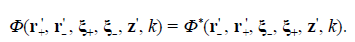
It has been shown that the kernel mode in Eq. (15) has a conical shape, and is a geometrical and deterministic function in the SM stage called the correlation cone (Castañeda et al., 2020). Its vertex is placed at the emission point, its basis covers a region of pairs of points (ξ +, ξ -) on the mask and exhibits a Lorentzian cross-section at any distance from the S plane (Figure 5a, b). It is apparent in Eq. (15) that the geometric attributes of the correlation cone are due to the non-paraxial Green's functions for the SM stage and are independent of the physical and statistical attributes of the effective source.
It is worth noting that the physical observable describing the arrival of the single particle at a given point of the M plane is the quantum probability

i.e., the local component of the prepared nonlocality. The kernel mode in Eq. (16) is a Lorentzian well with a vertex at the emission point whose geometrical shape is like that shown in figure 2a, b. Therefore, we can conclude that the correlation cone is a geometric deterministic condition established in the volume of the SM stage determined by its configuration. Its cross-section at the M plane gives the prepared nonlocality there independently of the single particle arriving at that plane, so once a single particle is locally emitted at the source plane, its movement towards the M plane (no matter the path it follows) is confined in the Lorentzian well in Eq. (16) and is also contained in the correlation cone in Eq. (15). Consequently, it arrives locally to any point in the cross-section of the Lorentzian well at the M plane, which is non-locally linked only with the other points enclosed by the cross-section of the correlation cone there. Given such specifically prepared non-local links, the corresponding geometric potential modes are activated in the MD stage. Thus, if a mask opening is placed at the arrival point, the geometric potential modes spatially modulate the individual Lorentzian well in the MD stage with the vertex at the mask opening. After crossing it, the particle movement toward the detector will be confined in such a spatially-structured Lorentzian well, and, therefore, the particle delocalization hypothesis is unnecessary.
An extended effective source is composed of a set of emission points with a quantum probability distribution that depends on the emission properties of the source. Each emission point is the vertex of an individual Lorentzian well and of a correlation cone, both in the SM stage. According to Eq. (14), the prepared nonlocality at the M plane results from the overlapping of all the correlation cones, no matter that only one emission point is active in each individual realization. Therefore, the size of the prepared nonlocality support at the M plane is reduced as the efective source size increases, as illustrated by the examples in figure 5c-f. Because of this reduction in the size of the prepared nonlocality support, modes of the geometric potential in the MD stage are filtered out, so that the confinement zones in this stage will not be strongly modulated and contrasted. This was evident in the experimental results of interference with single electrons (Matteucci et al., 2013) as a loss of the pattern visibility with single fullerene molecules (Nairz et al., 2003) with a cosine-like shape in the interference pattern, although a grating was attached at the M plane, and with other molecules (Juffmann et al., 2012) as a strong loss of contrast in the interference pattern. The analysis of these results in the framework of the current model was reported by Castañeda & Matteucci (2017).
Figure 5 Correlation cones in the SM stage for spatially incoherent optical sources or uncorrelated single massive particle sources attached at the S plane. Axial sections for 0 ≤ z ≤ 10λ (λ = 4pm for single matter particles and 4μm for light waves) on the left column and cross-sections at z = 10λon the right column for (a), (b) a point source, (c), (d) a source with two emission points, and (e), (f) an extended source with a regular array of five equivalent emission points with a spacing of a = λ/2. (ξ D , η D ) are the Cartesian coordinates of the separation vectors at the M plane. The nonlocality support is mainly determined by the central main maximum of the profiles and is centred in all cases at ξ A =0. The axes units are pm for single matter particles and μm for light waves.
This description is also valid for spatially incoherent optical fields, although all the emission points of the extended effective source can be continuously and simultaneously active, as fairly established by Wolf in his spatial coherence theory (Born & Wolf, 1993; Mandel & Wolf, 1995). Therefore, the Lorentzian well is completely filled by the source emissions, so that |ψ(r A ' ) |2 and |ψ(ξ A )|2 describe the irradiance distributions over the effective source and the mask, respectively.
This analysis emphasizes that the prepared nonlocality at the M plane seems not to be a physical or statistical property of the light or the single particles, but a condition established by the setup configuration. The influence of the spatial correlation properties of the effective source on the nonlocality preparation restricts to specifying and weighing the set of the non-local kernel modes in the integrand of Eq. (13).
Additionally, the local component of Eq. (13) specifies the physical observable w(ξ A , ξ A ) = |ψ(ξ A )|2 that describes the prepared distribution of the light irradiance or the single particles arriving at the M plane. It is the cross-section of the spatially-structured Lorentzian wells overlapped in the SM stage. The nonlocality properties of the effective source denoted by w(r’ + , r’ - ) activate the geometric potential that modulates the wells in the same way as in the MD stage with the prepared nonlocality at the mask. By following the same reasoning as in Eq. (6) and setting ξ D = 0, Eq. (13) yields |ψ(ξ A )|2 = |ψ(ξ A )|R 2 + Λ(ξ A ) with
and
whose phenomenological meanings in the context of the confinement principle for the SM stage are similar to those of the corresponding expressions for the MD stage given respectively by Eqs. (7) and (8).
Summarizing, the nonlocality function is geometrically prepared at the mask plane, i.e., its shape and size are closely related to the kernel modes, which are determined by the non-paraxial Green's functions for the SM stage, independently from the physical and statistical emission properties of the effective source. Nevertheless, such source features confer a statistical appearance to the recording of single particle arrivals and light irradiance by the detector without altering the geometry of the correlation cones and the spatially-structured confinement in the wells. This phenomenology in ordinary space clearly differs from the standard formalisms that describe nonlocality features in terms of the spatial correlation functions attributed to the light in free space or the representation of the particle beams in the Hilbert space.
¿Is the confinement entangled?
Since the notion of entanglement of quantum states was pointed out as a paradox by Einstein, Podolsky, and Rosen in a celebrated paper (Einstein et al., 1935), it has motivated strong discussions in different contexts of physics. For instance, it inspired the formulation of a hidden-variable theory (Bohm, 1952 a, b), a theorem to verify the existence of entanglement from experimental data (Bell, 1964), experiments to demonstrate its existence (Bohm & Aharonov, 1957; Freedman & Clauser, 1972; Aspect et al., 1982; Aspect, 2015), and contemporary technological perspectives (Paneru et al., 2020) including quantum computation, teleportation, quantum encryption, and telecommunications. In all these topics, as well as in the multiple scenarios in which different types of entanglement have been identified (Paneru et al., 2020), the notion of entanglement denotes non-separable quantum states of physical systems, such as photons and massive particles, for which the measurement on one state affects the other states without interaction between the systems (Bhaumik, 2018; Paneru et al., 2020), a behavior that Einstein called the "spooky action at a distance" (Born, 1971).
From the perspective of the proposed confinement principle for interference, the spatially-structured Lorentzian wells have been characterized as the behavior of free space related to (but independent from) the propagation of waves and massive particles between specific planes. More precisely, the Lorentzian wells are the behavior of ordinary space in the absence of prepared nonlocality at the input plane so the geometric potential is not activated. In the presence of prepared nonlocality, the activated geometric potential modulates the Lorentzian wells, thus establishing the spatially-structured wells.
Therefore, free space is regarded as a physical system that is able to confine the propagation of light energy as well as of single particles in spatially-structured wells. Furthermore, such wells characterize the geometrical states of free space whose attributes can be controlled by means of the prepared nonlocality. Consequently, a mask establishes a set of free-space geometrical states in the volume of the MD stage, each one corresponding to an individual Lorentzian well which is spatially structured by the subset of geometric potential modes activated by the prepared nonlocality. A peculiar feature of these states seems to approach the entanglement scenarios.
Let us consider the individual spatially-structured Lorentzian wells under strong nonlocality. As shown in section 2, each well must have forbidden regions (Figure 4) that reduce the confinement in the other wells, even to null at specific points. Thus, independent confinement regions are established in the complete spatially-structured well whose cross-section at the D plane gives a highly contrasted interference pattern. In other words, because of the spatial distribution of the forbidden regions in the individual wells, the set of free-space states is not separable, and the confinement in each one is affected by the other ones.
This can be clearly appreciated by considering the Young interference with a double pinhole mask with a separation vector a. Each individual Lorentzian well and the corresponding geometric potential are given, respectively, by the integrands of Eqs. (7) and (8), which can be denoted as |Γ(±a/2, r A , z, k)|2 and

with
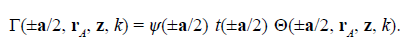
So, the cross-section of each individual spatially-structured Lorentzian well at the D plane is given by
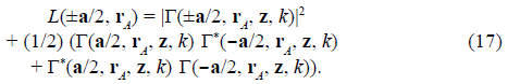
Equation (17) has remarkable mathematical and physical features. It is a non-factorable expression that is measurable at the points r A on the D plane and fulfills the condition L(+a/2, r A ) ≥ 0, in the sense that a squared modulus detector can record the confined light energy or the single particles at such points. The points r A for which L(+a/2, r A ) < 0 determines forbidden regions and the squared modulus detector cannot record light energy or single particles there. So, the "measurability" of L(+a/2, r A ) is ensured by the condition
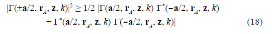
with

Nevertheless, the physical observable

is always measurable by a squared modulus detector. This indicates that the two individual spatially-structured Lorentzian wells L(±a/2, r A ) are non-separable to ensure the measurement of the interference pattern at the D plane and, additionally, |ψ(r A)|2 < L(±a/2, r A ) for L(∓a/2, r A ) < 0. This means that the forbidden regions of everyone well overlap the confinement regions of the other well. Consequently, the negative values of the forbidden zones of every well reduce the confinement in the other well.
Therefore, a peculiar behavior can be predicted. Let us start with a weak enough prepared nonlocality at the M plane, so that the forbidden zones are removed in the individual spatially-structured wells and L(±a/2, r A ) > 0. Under this condition, the two wells are separable in the sense that |ψ(r A )|2 can be determined by separated positive definite contributions measured at everyone well. The predicted outcome is a low contrasted interference pattern at the D plane for which |ψ(r A )|2 > L(±a/2, r A ). Now, let us increase the prepared nonlocality at the M plane. The geometry of the geometric potential mode remains invariant, but at the time when the forbidden zones appear in one of the individual wells, the confinement in the other well is reduced at the same place of the forbidden zone and in the same amount. This simultaneous effect in two different spatially-structured wells is caused by an action applied at a distant place, actually at the S plane of the SM stage, where the prepared nonlocality at the M plane is controlled. Furthermore, because of the mirror symmetry of the individual spatially-structured Lorentzian wells, the same reduction in confinement occurs symmetrically in both wells because of the appearance of symmetrical forbidden zones in them induced by the same geometric potential mode. Thus, the measurement of the reduced confined light energy or the single particles at a given point in one of the individual wells should reveal the simultaneous reduction of the confined light energy or the single particles by the same amount at the symmetric point in the other individual well.
This behavior of the Young interference is illustrated in figure 6a, c. The dotted line profiles are the cross-sections of the individual spatially-structured Lorentzian wells given by Eq. (17), and the continuous line profile results from their overlapping, as denoted in Eq. (19). Near the mask, the forbidden zones in both individual wells are denoted by the negative values of their profiles. It is worth noting that the confinement of each well is reduced in the segment coinciding with the forbidden zones of the other well, so that |ψ(r A )|2 takes on values between the individual profiles. In the far field, the forbidden zones reduce to null points of the profiles at the same positions on the D plane. It should be emphasized that this crucial feature of the geometric states of the space has not been explicitly described in the standard interference formalisms.
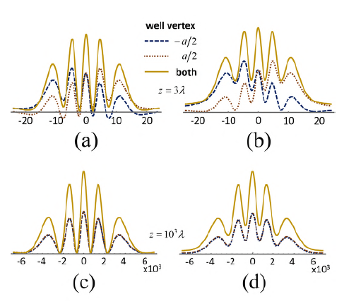
Figure 6 Spatial entanglement in Young interference. The cross-sections of the individual spatially-structured Lorentzian wells and their overlapping are shown (a) near the M plane and (c) in the far field. Removing the spatial entanglement by weakening the prepared nonlocality (b) near the M plane and (d) in the far field. The units are arbitrary.
The forbidden zones can be removed by weakening the nonlocality suitably, as shown in figure 6b, d. Consequently, the mutual influence on the confinement in each individual well disappears and the geometric states of the free space become separable, i.e., the confinement in each well only depends on its own spatial structure.
The analysis above suggests that a new type of entanglement involves the two spatially-structured Lorentzian wells that we call spatial entanglement. Such entanglement is controlled from outside the MD stage and manifests as the symmetrical reduction of the confinement in each well because of the forbidden zones in the other well. It should be noted that spatial entanglement is not a condition to build-up interference, but it is required for high-contrasted interference.
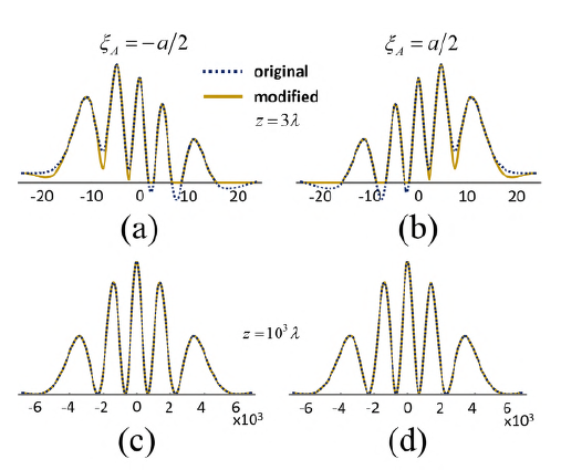
Physical observables describing the exact predictions of the confinement in the individual spatially-entangled wells can be obtained by simply adjusting the confinement zones in accordance with the forbidden zones as illustrated in figure 7. The predictions (continuous-line profiles) are compared with the original profiles of L(±a/2, r A ) (dotted-line profiles). Near the mask in (a) and (b), the forbidden zones of each L(±a/2, r A ) are set to null in the prediction profile, and their negative values are added to the confinement zones of the other well, so that the predicted values there become smaller than the profile values of L(±a/2, r A ). Outside the forbidden zones, the values of L(±a/2, r A ) predict the confinement in the well. This coincidence is complete in the far field, (c) and (d), where the forbidden zones of the individual wells reduce to only the null points of their cross-sections.
The measurement of the predicted confinement in spatially-entangled wells, as those illustrated in figure 7, should be regarded as a strong experimental challenge, not only because of the requirement of non-paraxial technology but also (and more importantly) because it involves measurements on the cross-section of each individual spatially-structured Lorentzian well. To make it possible, an experimental procedure different from the quantum eraser (Scully & Zubairy, 1997) should be implemented as this experiment precludes the simultaneous determination of the mask opening crossed by a particle, specifically a photon, and the detection of the interference pattern by the detector. Therefore, the quantum eraser setups are not suitable to verify the predictions depicted in figure 7, which renders this measurement extremely challenging.
Summary and conclusions
The phenomenology based on the novel principle of confinement in spatially-structured Lorentzian wells was discussed in detail. Its main advantage is to offer a unified and causal description of interference with classical waves and single massive particles in ordinary space. Instead of characterizing interference with waves and single particles by conferring them certain physical features, we assume the free space (or the field-free regions delimited by a setup) as a physical system with geometrical states capable of confining the light energy and the single particles in volumetric spatial structures whose cross-sections determine the interference patterns.
In contrast with the standard formalisms, this model accounts for individual experimental realizations where the emission, the crossing through the mask, and the detection are local events for both waves and particles. Nevertheless, a peculiar geometric feature of free space, called nonlocality, appears as the cause of interference. Instead of an attribute of the waves or the particles, nonlocality is prepared by the configuration of the setup. Furthermore, by strongly prepared nonlocality, the free-space geometrical states seem to become spatially entangled, i.e., the forbidden zones of each individual spatially-structured Lorentzian well affect the confinement in the other individual wells, thus ensuring the build-up of high-contrasted interference patterns. The spatial entanglement is removed by suitably weakening the prepared nonlocality.
It should be emphasized that this model is rigorously based on the solution of the Helmholtz equation (i.e., the spatial component of both the classical wave equation for free space and the Schròdinger equation for field-free regions) using Green's theorem, and relates Green's function to the geometric states of free space. It seems to be the starting point of its departure from the standard classical and quantum formalisms of interference without affecting its accuracy in predicting experimental outcomes.
So, in the phenomenology of the confinement in spatially-structured Lorentzian wells, duality hypotheses like particle delocalization and self-interference are unnecessary. A further important feature of the proposed model is the simultaneous presence of the Lorentzian wells and the correlation cones in the volume of the preparation stage of the setup. Following the same reasoning, it can also be established in the measurement stage. It should be underlined that this feature questions the requirement of wave function "collapse" as the local measurement of the arrival of a single particle at the detector is performed. Indeed, squared modulus detectors perform local measurements only on the cross-section of the Lorentzian well without affecting the nonlocality in the detection area and demand that the eigenfunction does not nullify when the local measurement is performed.

