


 English (pdf)
 Article in xml format
 Article references
 Send this article by e-mail
 Cited by SciELO
  Cited by Google
  Similars in
SciELO
Similars in
SciELO  Similars in Google
 Permalink
INTRODUCTION
The southeast region of Mexico is characterized by significant social backwardness and high levels of poverty and illiteracy (Dávila, Kessel & Levy, 2002), accompanied by a low level of economic growth. Given the economic and social backwardness that exists in this region, Esquivel, López & Vélez (2003) argue that investment policies focused on human capital and infrastructure are priorities.
Public infrastructure, being a productive investment, is fundamental to stimulate the economic dynamics of a region because it is the base on which diverse activities are supported, thus promoting economic growth. Increased availability and a higher quality of infrastructure lead to higher factor productivity and lower production costs (Aschauer, 1990). In contrast, their absence is a major obstacle to the effective implementation of development policies and, with this, the achievement of levels of sustainable growth (World Bank, 1994).
The objective of this paper is to estimate the impact of public infrastructure (social and economic) on the economic growth of the eight regions of Oaxaca, Mexico for the period 2003-2013. Consistent with the characteristics and rugged topography of Oaxaca, the work suggests what types of infrastructure are appropriate for each of the regions.
This remainder of this article is structured as follows: Section I is a review of the literature. Section II presents the methodology proposed by Gerber (2003) to calculate regional growth rates. Section III estimates the impact of infrastructure on growth based on the approach used by Hoechle (2007), augmented with a fixed effects model. Section IV presents the conclusions.
1. PUBLIC INFRASTRUCTURE: A REVIEW OF LITERATURE
For Aschauer (1990) the government fulfills two functions: it collects taxes and it provides public goods (services). The public goods are divided into consumer-oriented goods (parks, museums, etc.) and goods dedicated to production (for example, the construction and maintenance of roads). The latter, also considered productive goods, have a double function: they can function as intermediate inputs or as final inputs. In the literature (Aschauer, 1989; Aschauer, 1990; Munnell, 1990a; Fuentes, 2003; Noriega & Fontenla, 2007; Hernández, 2009, 2010), there is a consensus that public infrastructure is a factor that explains long-run economic growth.
1.1. Types of infrastructure
There is no widely-accepted definition ofpublic infrastructure. For Hirschman (1958) it includes those basic services without which there could be no primary, secondary and tertiary productive activities. In its broadest sense it includes all public services, from education and public health to transport, communications and the supply of energy and water. It is a set of public assets that generates an environment where social interaction and economic processes take place (Piedras, 2003). According to Diamond (1990), infrastructure has three basic characteristics: (a) it is a collective input; (b) it includes investments in both physical capital and human capital; and (c) it is integrative; the components are integrated through telecommunications networks, transport, and transactions.
Because of its characteristics and functions, public infrastructure is a good that is not normally supplied by the market or that only supplies it inefficiently, so that its provision is fundamentally determined by political decisions (Biehl, 1988). Fuentes (2003) mentions that infrastructure can be classified into three categories: material (or physical), institutional, and personal. The first element is understood as the stock ofpublic capital (roads, water dams, schools, etc.) produced and administered by the State to be used by companies and households, which contributes to the production process. The institutional infrastructure is the set of norms, institutions and procedures designed by the State that determine the framework within which economic agents interact with each other. Finally, personal infrastructure includes the size and structure of the active population and its productive capacities.
The varying context, characteristics, and even the availability of information in a geographical area have led different authors to define and categorize the infrastructure according to their objectives. In this analysis we follow Hansen (1965) 1 and Aschauer (1989), who separate physical infrastructure into social and economic elements. The social category is aimed at improving the welfare of individuals, in the areas of education, health, and culture and indirectly increases productivity. The economic category is directly oriented to productive activities or to the movement of economic goods, which includes roads and telecommunications.
1.2. Theoretical model
A model that analyzes the impact of public infrastructure on economic growth is presented by Aschauer (1990). The production model is of the Cobb-Douglas type:

where Y refers to the level of output within the jurisdiction, K is private capital, G represents government spending on productive infrastructure, L is the labor force, and A is the index of technological progress. It is assumed that this production function presents constant returns to scale.
By transforming (1) in terms of per capita and linearizing the equation, we obtain
where the lowercase letters denote the logarithms of the variables. We assume that capital is a mobile factor and that it flows between the jurisdictional limits; such that, at least in the long term, the marginal product of private capital is equal among jurisdictions. Therefore, the marginal product of capital and the elasticity of the product with respect to capital are given by
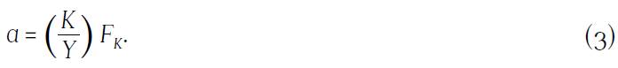
Equation (3) indicates that the differences in the elasticity will be reflected in the differences in the capital-output ratios. Likewise, the marginal product of the productive infrastructure and the elasticity of the product with respect to these services are given by

We assume that the public agent chooses a level of public goods consistent with the marginal productivity of the infrastructure in the particular geographical area. Consequently, the differences in the levels of services provided by the government are reflected in differences in the production function in the respective geographical regions.
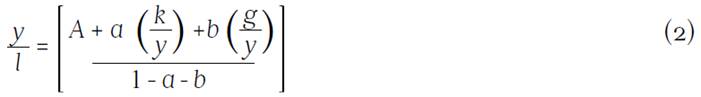
Substituting the elasticity of equations (3) and (4) in the production function in (2) we have:
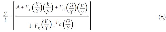
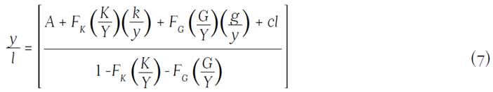
Equation (5) is the one used to estimate the impact of infrastructure on economic growth. However, this equation assumes that infrastructure only works for one industry. When it is considered that the infrastructure is used by more than one user (that is, it is a non-rival good), the production function (1) is rewritten as

In this case, if c = 0, the production function will be characterized by having constant returns to scale in all productive inputs. If c = 1, it will be characterized by having constant returns in private inputs, with the implication of increasing returns in the private and public inputs. Therefore, in this case, the function to estimate is
1.3. Empirical literature
The economic effects generated by physical infrastructure in the literature differ in quantitative terms. This is due to the fact that different authors use different data and methodologies (monetary units, physical units, production function, cost function, etc.), together with the fact that they define infrastructure differently. However, most of them agree that public infrastructure has a positive effect on employment, the productivity of the private sector, the total productivity of factors and, therefore, on economic growth. For example, García (2007) reviews the literature and concludes that there is evidence of a positive relationship between investment in transportation infrastructure and economic growth. In addition, public infrastructure generates positive externalities (Duque, Velásquez & Agudelo, 2011).
Aschauer (1989) performs a case study of the United States for the period 1949-1985, which shows that the impact of productive public capital on private production and on the total productivity of the factors is significant; in precise terms a 1% increase in public infrastructure generates an increase in the gross domestic product (GDP) per capita of 0.24%. Likewise, in a disaggregated analysis he shows that the economic infrastructure has a close relationship with productivity, with an elasticity of 0.24. In a similar analysis Munnell (1990a) mentions that the increase in GDP is 0.35%, and further that the infrastructure determines the location of companies. In other research Aschauer (1990) and Munnell (1990b) argue that the decline in productivity suffered by the United States in the 1970s was due to a fall in the rate of investment in public capital. The effect of infrastructure on GDP decreases as the level of geographic disaggregation increases. At the aggregate level the impact is 0.3% (Aschauer, 1998); at the state level, the effect on growth varies between 0.15% (Munnell, 1990a) and 0.20% (Costa, Ellson & Martin, 1987); and at a local level, Duffy-Deno & Eberts (1991) find an effect of 0.08%.
The difference in infrastructure endowments causes regional disparities in GDP per capita, thus widening the amount of divergence (Peña, 2008). Argimón, Gonzalez, Martin & Roldan (1994) and Delgado & Álvarez (2000) point out that investment in public capital in infrastructure improves (complements) and has a positive impact on the productivity of the Spanish private sector. For De la Fuente (2008) infrastructure is a mechanism of redistribution, which has led to the convergence of Spanish regions and generated accessibility for lagging regions. In Colombia, Mendoza and Yanes (2014) find that in medium and large regions, the dynamics of public investment explain their economic growth.
Chinese provinces differ in terms of reforms, transparency, geographical location, and, above all, in the provision of infrastructure. These elements have caused the differences in regional productivity (Démurger, 2001). Rama (1993), in a study applied to underdeveloped countries (including Mexico), finds a “crowding out” effect of public investment over private investment. In contrast, Cardoso (1993) and Ramírez (1994) argue that, in the aforementioned relationship, the “crowding in” effect predominates; that is, public investment complements private investment. In a study made to a group of countries, it is pointed out that the elasticity of GDP per capita with respect to infrastructure is not clear (Calderón, Moral-Benito & Servén, 2015).
In Mexico for the period after 1982, authors such as Lächler & Aschauer (1998) link, in part, the deceleration of economic growth with a decrease in public investment. Hernández (2011) points out that the adverse effects of public intervention, which gave rise to the debt crisis of the 1980s, caused a contraction of the share of the public sector in the economy, that is, the Mexican State abandoned its function of promoter of development (Torres & Rojas, 2015). Since the 1980s, Mexico has exhibited a fall in productivity (Piedras, 2003) and, therefore, a slow rate of growth. One of the factors involved is a drop in the rate of public investment, particularly in infrastructure (Ros, 2008).
Mexico is a country of great contrast between the states of the north and south that is manifested through the disparities in per capita income, education, and social welfare. A factor that explains the income inequality between different geographical areas is infrastructure endowment (Argimón et al., 1994); which as a result of inappropriate regional public policies were not focused on the needs of each region (Fuentes, 2003).
For Aschauer (1998) the structural reforms that were applied in Mexico as part of the fiscal austerity program reduced the level of growth of public capital. Lächler & Aschauer (1998) suggest that the government should restructure public spending, assigning greater emphasis to public investment. Noriega & Fontenla (2007) affirm that investment in infrastructure is complementary to private investment and that in the long term increases in infrastructure in the categories of electricity supply and roads have positive effects on GDP per capita.
The effects of public investment at the state level in Mexico have been studied by several authors (Fuentes, 2003; Fuentes & Mendoza, 2003; Costa-i-Font & Rodríguez, 2005), who point out that although the different national development plans have aimed to reduce economic inequality between regions, differences have continued due to the disparities in the provision of infrastructure. That is, infrastructure has focused on a few entities (especially in manufacturing), which has given certain regions more dynamism (Tamayo, 2001). For the State of Mexico, Vergara, Mejía & Martínez (2010) indicate that only the social infrastructure conditions the growth rate among the municipalities. On the other hand, Barajas & Gutiérrez (2012) show that the economic infrastructure is important for border municipalities given their close economic relationship with the United States, showing an elasticity of physical and economic infrastructure with respect to the per capita product of 0.38%. In summary, physical infrastructure reduces inequality and raises the standard of living, while at the same time performing distribution functions (Calderón & Servén, 2004; World Bank, 1994).
2. TREATMENT OF DATA
To estimate the impact of infrastructure on the economic growth of the regions of Oaxaca2 it is necessary to have disaggregated data, both on infrastructure and economic output. In the case of output information is only available at the state level, provided by the Mexican National Institute of Statistics and Geography (INEGI).
2.1. Estimation of regional GDP per capita
To estimate GDP per capita in the regions of Oaxaca, we follow the methodology proposed by Gerber (2003). The author assumes that there is the same level of productivity within a given sector and between the regions of a given state. The regional product is measured through the participation of each sector in the state GDP and the employment share of each region in state employment.3 From these participations we obtain a parameter (λ) that indicates the role of the region in the state economy

where Ys i represents state income in sector i, Ys is state income, er i indicates regional employment in sector i, es i is state employment in region i. The regional GDP (Yr ) is obtained by multiplying the product of equation (8) by the state GDP

To calculate the employed population for the 2003-2013 periods, approximations of state and regional employment were made by interpolating the 2004, 2009 and 2014 Economic Censuses to obtain equation (9) on an annualized basis. The estimation was made following the methodology used by Mendoza (2006):
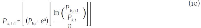
where P is the employed population, a is the year, and t refers to the base year.
Economic growth per capita in the state of Oaxaca is heterogeneous (Table 1). The regions have been growing irregularly and exhibit enormous differences in levels of well-being. Only two regions (the Istmo and the Valles Centrales) have acceptable standards of living, above the value specified by the state. The Cañada, Sierra Norte, Sierra Sur and Costa regions show the lowest levels, so they can be considered the most lagging regions.4 These regions have had average annual growth per capita levels between 8 and 11 percent; this is explained by the decrease in the population in these regions.
The changes in the regions of the Istmo and Valles Centrales (those with the lowest average growth in the last decade) can be explained by the fact that in these regions the growth rate of the economic output does not compensate for the rate of population growth. However, despite the above, it can be observed that for the last year of study (2013), economic inequality, in terms of GDP per capita, had been reduced compared to 2003. In 2003 the value of the GDP per capita of the region of the Valles Centrales was more than eight times the value in the Cañada region. However, for 2013 inequality was reduced to only 3.5 times. According to the estimations, the Istmo and Valles Centrales regions, as a whole, have a share of approximately 70 percent of the state per capita GDP. These two regions have more than 60% of the occupied population of the entity. In terms of their economic structure, these regions show similar behavior to the state (Table 2).
Table 1 Oaxaca: Estimation of regional GDP per capita 2003-2013 (2008 pesos)
| 2003 | 2004 | 2005 | 2006 | 2007 | 2008 | 2009 | 2010 | 2011 | 2012 | 2013 | |
| Cañada | 9.638 | 10.678 | 11.492 | 12.143 | 12.851 | 13.436 | 14.104 | 15.418 | 16.991 | 18.814 | 20.457 |
| Costa | 27.803 | 29.594 | 30.691 | 31.464 | 32.205 | 31.959 | 31.868 | 33.133 | 33.387 | 34.242 | 34.629 |
| Istmo | 59.709 | 59.981 | 59.294 | 58.969 | 58.511 | 57.110 | 55.563 | 55.632 | 55.678 | 56.114 | 57.067 |
| Mixteca | 29.312 | 31.448 | 32.934 | 33.393 | 34.089 | 34.349 | 34.960 | 37.090 | 39.484 | 41.645 | 41.668 |
| Sierra Sur | 12.504 | 14.049 | 15.611 | 16.913 | 18.594 | 20.387 | 20.192 | 21.475 | 23.510 | 26.283 | 27.547 |
| Sierra Norte | 12.861 | 13.936 | 14.659 | 14.929 | 15.300 | 15.824 | 17.205 | 20.352 | 24.880 | 31.038 | 35.528 |
| Papaloapan | 34.081 | 35.253 | 35.783 | 36.328 | 36.826 | 36.691 | 34.592 | 33.427 | 32.357 | 31.368 | 30.343 |
| Valles Centrales | 81.894 | 82.757 | 81.953 | 80.774 | 79.968 | 79.320 | 75.951 | 74.314 | 74.941 | 74.728 | 73.258 |
Source: Own estimates based on data from XII General Population and Housing Census (2000) and Population and Housing Census (2010); Count of Population and Dwellings, 2005; Economic Censuses 2004, 2009, 2014; System of National. Accounts of Mexico; and Conapo, Projections of the population of Mexico 2010-2050.
Table 2 Oaxaca: share (%) of the population occupied by region and economic sector (2003-2013)
| 2003 | 2008 | 2013 | |||||||
| Primary* | Secondary | Tertiary | Primary* | Secondary | Tertiary | Primary* | Secondary | Tertiary | |
| Estatal | 3,05% | 21,11% | 75,84% | 1,60% | 14,84% | 83,57% | 1,22% | 24,04% | 74,75% |
| Cañada | 1,55% | 26,84% | 71,61% | 1,46% | 16,76% | 81,78% | 0,77% | 23,62% | 75,61% |
| Costa | 5,31% | 10,15% | 84,54% | 3,90% | 6,42% | 89,68% | 3,29% | 16,64% | 80,06% |
| Istmo | 8,76% | 24,31% | 66,93% | 3,69% | 17,48% | 78,83% | 3,83% | 39,69% | 56,49% |
| Mixteca | 0,23% | 16,27% | 83,50% | 0,28% | 13,83% | 85,89% | 0,06% | 18,48% | 81,47% |
| Sierra Norte | 0,37% | 27,70% | 71,93% | 0,94% | 20,02% | 79,03% | 0,17% | 13,40% | 86,43% |
| Sierra Sur | 0,00% | 27,78% | 72,22% | 0,48% | 17,19% | 82,33% | 0,06% | 7,59% | 92,35% |
| Papaloapan | 6,69% | 25,14% | 68,17% | 4,04% | 15,58% | 80,37% | 4,60% | 31,28% | 64,12% |
| Valles Centrales | 0,00% | 21,17% | 78,83% | 0,03% | 15,30% | 84,67% | 0,02% | 36,73% | 63,25% |
Note:* The sector managed as primary in the Economic Censuses only includes fishing and aquaculture activities, leaving aside the activities of agriculture, livestock and forestry. Source: Own elaboration based on Economic Censuses 2004, 2009 and 2014.
2.2. Infrastructure index
Infrastructure can be quantified in monetary or physical units (Delgado & Álvarez, 2001; Fuentes, 2003; Becerril, Álvarez, Del Moral & Vergara, 2009). The use of monetary units presents a disadvantage; it does not present a direct relationship between investment costs and service capacity (Biehl, 1988; Cancelo & Uriz, 1994). For example, the rugged terrain of a state such as Oaxaca may skew the costs of infrastructure construction, which would imply an overestimate of infrastructure endowments.
In the case of physical units, the infrastructure can be measured with partial or synthetic indicators. The first refers to the type of unit of measure for each category or subcategory of infrastructure (for example, roads are measured in kilometers); meanwhile, for the latter complex indices are produced that show the capacity of the equipment. However, since there are different units of measurement for the infrastructure (in kilometers, in units, etc.), it is necessary to establish a method of aggregation (Delgado & Álvarez, 2001; Fuentes & Mendoza, 2003). For synthetic indices the main advantage is that, in addition to avoiding problems of overestimation, it provides a large amount of useful information for detailed evaluations (Becerril et al., 2009). The indicators used in this work are shown in Table 3. Following Fuentes (2003), the physical indicator as a whole is called the Global Infrastructure Index (IGI). It is composed of two categories: economic productive infrastructure (IPE) and productive social infrastructure (IPS).
Table 3 Description of indicators
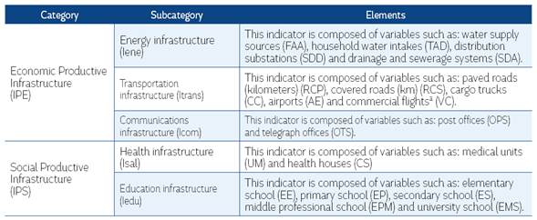
Source: Own elaboration based on Fuentes (2003) and Barajas & Gutiérrez (2012), with information from the Statistical Yearbooks of Oaxaca (several years) and the Mexican National Institute of Statistics and Geography (INEGI). In parentheses the nomenclature used in the database. a The latter are used as a measure of the capacity of roads and airports.
For the elaboration of infrastructure indices, each of the variables is normalized. If this is not done, the larger the region (geographic or population dimension), the greater the infrastructure endowment in absolute terms, which will exaggerate the differences between the regions. This transformation of the variables is necessary to homogenize the regions (Delgado & Álvarez; 2001; Cancelo & Uriz, 1994).
The adjustment for the size of the region is performed by using the total population of each region as a reference measure of its geographic area:

where a i,k is the infrastructure equipment for variable i in region k, W i, k represents the original magnitudes for each variable i in region k, S k is the geographical area (km) of the region k and P k corresponds to the total population of the region k.
Given that the units in which these variables are expressed are not comparable, the subsequent procedure normalizes the variables and makes the values one-dimensional and comparable (Cancelo & Uriz, 1994; Delgado & Álvarez, 2001):

where a i,k refers to infrastructure equipment for variable i in region k, a MAX represents the measure of region with the maximum value, and S i, k is a standardized indicator for variable i in the region k.
The next step is to apply a data aggregation procedure that synthesizes the information. One of the methods used is that of Beihl (1988), who mentions that for the aggregation of the variables in each subcategory, arithmetic means must be used, because with this procedure the lower endowments of some types of equipment can be compensated with higher endowments of others due to the substitutability effect (Delgado & Álvarez, 2001). The aggregation of synthetic indicators Biehl (MB) (Cancelo & Uriz, 1994) is constructed, for each category, by means of an arithmetic mean of the following form:

where I j, k is the indicator of category j in region k and S i, k represents the normalized indicator for variable i in region k.
The categories are added with a geometric mean since they are irreplaceable (Biehl, 1988). The formulation is the following:
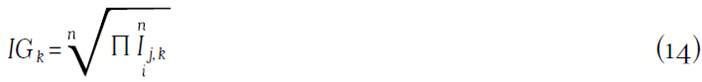
where IG k is the global indicator of infrastructure in the region k. This index allows to eliminate possible effects of magnitude, for example, of length when measuring the transport infrastructure.
In order to contrast the situation of Oaxaca with respect to other states, we developed an indicator of physical infrastructure for each of the states of Mexico (Table 4). Among Mexican states Oaxaca’s relative position depends on the index examined. When using the population-weighted indices, that is, indices per capita, Oaxaca is in a favorable situation with respect to the rest of the states in terms of infrastructure endowment (global infrastructure index). The element that explains this result is the low rate of population growth that the state has experienced in the last decade.
However, when the geographic area (km2) of each state is used to homogenize the data, the situation in Oaxaca is different from that indicated in the previous paragraph. In other words, when considering the infrastructure variables in terms of endowment per km2, both in the IGI and in the respective categories (IPS and IPE), Oaxaca has values below the national average because the Oaxaca localities are territorially dispersed, which means that coverage is minimal (Table 4).
Table 4 Oaxaca: provision of public infrastructure 2003 and 2013
| 2003 | ||||||||
| Isal | Iedu | IPS | Iene | Itrans | Icom | IPE | IGI | |
| Per capita | 89 | 57,97 | 71,83 | 26,75 | 34,6 | 51,79 | 36,33 | 51,08 |
| National average | 36,79 | 43,7 | 39,39 | 36,12 | 32,79 | 36,97 | 33,79 | 35,68 |
| By Km2 | 26,47 | 12,34 | 18,07 | 5,68 | 20,56 | 20,59 | 13,4 | 15,56 |
| National average | 20,4 | 20,4 | 20 | 14,8 | 29,23 | 26,9 | 21,4 | 20,2 |
| 2013 | ||||||||
| Per capita | 97,66 | 62,25 | 77,97 | 51,78 | 30,56 | 89,2 | 52,06 | 63,71 |
| National average | 42 | 44,8 | 42,7 | 39 | 30,5 | 36,8 | 34,4 | 37,8 |
| By Km2 | 31,19 | 11,31 | 18,78 | 15,82 | 14,6 | 40,95 | 21,15 | 19,93 |
| National average | 24,2 | 19,3 | 21 | 18,9 | 24,95 | 26,9 | 22,7 | 21,6 |
Source: Own elaboration.
At the regional level, applying the aforementioned methodology, we obtained the infrastructure indices for each category (social and economic) and global on a per capita basis. It is important to clarify that with this index when a region has a high index value (close to 100), it does not mean it has reached the optimal level of investment, rather that it is in a better position of infrastructure endowment with respect to other regions.
Table 5 Oaxaca: Global Infrastructure Index per capita: 2003-2013
| Region | 2003 | 2004 | 2005 | 2006 | 2007 | 2008 | 2009 | 2010 | 2011 | 2012 | 2013 |
| Cañada | 40,18 | 40,53 | 40,17 | 39,81 | 40,65 | 39,62 | 41,65 | 41,46 | 41,5 | 40,27 | 41,96 |
| Costa | 49,68 | 50,58 | 51,38 | 50,87 | 51,08 | 49,09 | 51,45 | 50,44 | 49,42 | 50,26 | 50,59 |
| Istmo | 41,67 | 41,91 | 40,98 | 41,61 | 38,61 | 37,86 | 38,27 | 37,85 | 37,08 | 37,11 | 37,29 |
| Mixteca | 58,69 | 60,46 | 59,88 | 60,35 | 58,24 | 56,21 | 57,53 | 56,31 | 56,12 | 52,44 | 54,76 |
| Papaloapan | 78,93 | 80,22 | 82,08 | 78,85 | 81,76 | 82,29 | 82,89 | 82,03 | 80,93 | 82,25 | 81,37 |
| Sierra Norte | 48,75 | 50,8 | 51,29 | 52,43 | 50,66 | 44,03 | 51,42 | 50,81 | 46,26 | 46,68 | 46,7 |
| Sierra Sur | 21,27 | 21,52 | 21,28 | 20,1 | 21 | 20,46 | 20,81 | 20,83 | 20,02 | 19,86 | 20,44 |
| Valles Centrales | 36,05 | 35,09 | 35,52 | 34,6 | 31,22 | 30,77 | 31,24 | 30,69 | 31,26 | 29,62 | 29,29 |
Source: Own elaboration based on INEGI, the Statistical Yearbooks of Oaxaca (several years).
The indicator of global infrastructure for each of the regions is presented in Table 5. It can be observed that the evolution of the infrastructure endowment in this decade of study has not been as favorable for the Istmo and the Valles Centrales regions where the index declined by approximately 11 and 19 percent, respectively. One of the causes of the reduction in the index of public infrastructure was the high rate of population growth. These regions stand out from the others due to their attractive economic dynamics (the second more than the first), which encouraged population growth. Other regions such as the Mixteca, the Sierra Norte and the Sierra Sur also show a decrease, although to a lesser extent than the two mentioned above.
Table 6 Oaxaca: Social Productive Infrastructure Index per capita: 2003-2013
| Region | 2003 | 2004 | 2005 | 2006 | 2007 | 2008 | 2009 | 2010 | 2011 | 2012 | 2013 |
| Cañada | 49,13 | 47,02 | 46,58 | 46,72 | 47,44 | 44,3 | 48,26 | 49,53 | 50,18 | 50,85 | 51,07 |
| Costa | 44,9 | 44,4 | 43,66 | 44,32 | 43,52 | 40,08 | 44,67 | 44,36 | 44,36 | 43,57 | 43,25 |
| Istmo | 33,5 | 33,6 | 32,31 | 33,37 | 32,94 | 31,08 | 32,63 | 33,37 | 33,68 | 33,27 | 33,27 |
| Mixteca | 55,72 | 55,57 | 54,04 | 55,7 | 54,33 | 50,11 | 52,61 | 52,36 | 52,29 | 48,18 | 52,5 |
| Papaloapan | 89,44 | 89,44 | 89,44 | 89,44 | 89,44 | 89,44 | 89,44 | 89,44 | 89,44 | 89,44 | 89,44 |
| Sierra Norte | 50,78 | 50,38 | 49,68 | 51,54 | 50,81 | 46 | 52,8 | 52,59 | 52,7 | 52,48 | 52,28 |
| Sierra Sur | 18,55 | 18,07 | 17,88 | 17,65 | 17,83 | 16,36 | 16,97 | 16,95 | 16,86 | 16,62 | 16,69 |
| Valles Centrales | 27,04 | 26,04 | 25,61 | 24,88 | 23,86 | 22,8 | 24,71 | 24,7 | 24,79 | 22,75 | 22,67 |
Source: Own elaboration based on INEGI, the Statistical Yearbooks of Oaxaca (several years).
Table 6 shows the index of productive social infrastructure. With the exception of the region Papaloapan, which has maintained a constant endowment (the best-positioned), and Cañada and Sierra Norte, which had a slight increase, most regions have shown a downward trend. Regarding the productive economic infrastructure (Table 7), the situation is not so different from the previous patterns. The Cañada, Costa, Papaloapan and Sierra Sur regions have shown a positive evolution. In the rest of the regions, the decrease is more pronounced in this index than in the global index and in the social indicator. The decrease in the indicators, which have been shown by the regions with a greater share of the state product, Valles Centrales and Istmo, is a sign that in these areas greater investment in public infrastructure is needed to facilitate the mobility of inputs and goods and an increase in factor productivity.
Table 7 Oaxaca: Economic Productive Infrastructure Index per capita: 2003-2013
| Region | 2003 | 2004 | 2005 | 2006 | 2007 | 2008 | 2009 | 2010 | 2011 | 2012 | 2013 |
| Cañada | 32,86 | 46,8 | 34,64 | 33,92 | 34,83 | 35,44 | 35,95 | 34,71 | 34,32 | 31,89 | 34,47 |
| Costa | 54,96 | 24,4 | 60,47 | 58,38 | 59,96 | 60,12 | 59,26 | 57,35 | 55,06 | 57,97 | 59,18 |
| Istmo | 51,83 | 48,08 | 51,98 | 51,88 | 45,25 | 46,13 | 44,89 | 42,92 | 40,82 | 41,38 | 41,79 |
| Mixteca | 61,82 | 34,93 | 66,34 | 65,38 | 62,45 | 63,07 | 62,92 | 60,55 | 60,23 | 57,08 | 57,12 |
| Papaloapan | 69,65 | 57,62 | 75,33 | 69,51 | 74,74 | 75,71 | 76,82 | 75,24 | 73,22 | 75,63 | 74,03 |
| Sierra Norte | 46,8 | 52,27 | 52,95 | 53,34 | 50,51 | 42,14 | 50,07 | 49,09 | 40,61 | 41,52 | 41,71 |
| Sierra Sur | 24,4 | 65,78 | 25,33 | 22,88 | 24,73 | 25,58 | 25,51 | 25,6 | 23,77 | 23,74 | 25,03 |
| Valles Centrales | 48,08 | 71,95 | 49,27 | 48,12 | 40,84 | 41,54 | 39,49 | 38,13 | 39,43 | 38,56 | 37,85 |
Source: Own elaboration based on INEGI, the Statistical Yearbooks of Oaxaca (several years).
Using the geographic dimension (square kilometer) as an element that eliminates the size effect, a change is observed with respect to the per capita indices. In this case, the Valles Centrales region becomes the region with the best infrastructure.
Table 8 Oaxaca: Global Infrastructure Index per km2: 2003-2013
| Region 2003 2004 2005 2006 2007 2008 2009 2010 2011 2012 2013 | |||||||||||
| Cañada | 59,34 | 59,54 | 58,75 | 58,69 | 62,52 | 62,66 | 62,91 | 64,63 | 60,12 | 55,81 | 59,45 |
| Costa | 59,4 | 61,34 | 61,3 | 61,34 | 64,15 | 64,5 | 65,35 | 65,63 | 63,34 | 66,23 | 66,87 |
| Istmo | 30,72 | 31,03 | 30,52 | 31,11 | 29,74 | 29,77 | 29,17 | 29,73 | 28,9 | 29,18 | 29,35 |
| Mixteca | 49,68 | 50,69 | 50,17 | 50,4 | 51,14 | 51,28 | 51,24 | 52,17 | 49,16 | 45,95 | 48,27 |
| Papaloapan | 48,46 | 47,81 | 48,43 | 47,91 | 51,24 | 53,82 | 52,9 | 54,9 | 52,19 | 52,19 | 51,61 |
| Sierra Norte | 28,36 | 30,07 | 30,1 | 30,68 | 31,63 | 29,91 | 32,27 | 32,99 | 30,13 | 30,38 | 30,35 |
| Sierra Sur | 35,7 | 35,28 | 34,98 | 33,53 | 35,62 | 35,43 | 35,71 | 37,11 | 34,57 | 33,94 | 35,32 |
| Valles Centrales | 83,43 | 83,96 | 84,21 | 83,88 | 84,39 | 84,89 | 83,33 | 83,52 | 84,35 | 84,56 | 84,22 |
Source: Own elaboration based on INEGI, the Statistical Yearbooks of Oaxaca (several years).
In the IGI, the regions of the Istmo, Mixteca and Sierra Sur showed a decline over time, although not significant (Table 8). In the case of social infrastructure, the evolution of this indicator is positive, with the exception of Sierra Sur, which declined (Table 9). This indicates that the infrastructure in health and education has increased in each of the regions. The economic infrastructure follows a behavior similar to the global indicator, being, in the same way, Valles Centrales the best-positioned region (Table 10). This region contains the capital of the State and is where there is a greater economic dynamic. However, it shows a downward trend together with regions such as Cañada, Istmo and Mixteca.
Table 9 Oaxaca: Social Productive Infrastructure Index per km2: 2003-2013
| Region | 2003 | 2004 | 2005 | 2006 | 2007 | 2008 | 2009 | 2010 | 2011 | 2012 | 2013 |
| Cañada | 84,24 | 84,5 | 84,03 | 84,34 | 84,27 | 84,71 | 85,13 | 85,9 | 86,19 | 86,92 | 86,9 |
| Costa | 65,43 | 67,71 | 67,37 | 68,6 | 68,75 | 69,65 | 69,77 | 69,47 | 70,18 | 70,71 | 70,69 |
| Istmo | 28,3 | 29,44 | 28,98 | 30 | 29,97 | 29,83 | 28,97 | 29,51 | 29,78 | 30,5 | 30,62 |
| Mixteca | 53,31 | 55,1 | 54,21 | 55,37 | 55,3 | 54,76 | 53,8 | 53,5 | 53,49 | 49,67 | 55,28 |
| Papaloapan | 63,03 | 65,67 | 65,63 | 66,47 | 66,27 | 72,37 | 67,67 | 67,53 | 67,91 | 68,48 | 68,81 |
| Sierra Norte | 35,61 | 36,85 | 36,74 | 37,97 | 38,49 | 38,4 | 39,23 | 39,24 | 39,58 | 40,49 | 40,54 |
| Sierra Sur | 36,71 | 37,52 | 37,53 | 37,27 | 37,52 | 36,22 | 36,06 | 35,79 | 35,64 | 35,36 | 35,7 |
| Valles Centrales | 78,09 | 79,3 | 79,62 | 79,57 | 80,55 | 80,92 | 78,81 | 79,01 | 79,75 | 80,63 | 81,2 |
Source: Own elaboration based on INEGI, the Statistical Yearbooks of Oaxaca (several years).
Table 10 Oaxaca: Economic Productive Infrastructure Index per km2: 2003-2013
| Region | 2003 | 2004 | 2005 | 2006 | 2007 | 2008 | 2009 | 2010 | 2011 | 2012 | 2013 |
| Cañada | 41,81 | 22,59 | 41,08 | 40,85 | 46,39 | 46,34 | 46,5 | 48,63 | 41,94 | 35,84 | 40,67 |
| Costa | 53,93 | 34,71 | 55,77 | 54,85 | 59,86 | 59,74 | 61,2 | 62,01 | 57,17 | 62,04 | 63,26 |
| Istmo | 33,36 | 89,14 | 32,14 | 32,27 | 29,52 | 29,72 | 29,39 | 29,96 | 28,04 | 27,93 | 28,14 |
| Mixteca | 46,3 | 41,95 | 46,43 | 45,87 | 47,28 | 48,03 | 48,8 | 50,88 | 45,19 | 42,51 | 42,15 |
| Papaloapan | 37,26 | 55,57 | 35,74 | 34,53 | 39,61 | 40,02 | 41,35 | 44,63 | 40,11 | 39,77 | 38,72 |
| Sierra Norte | 22,59 | 32,71 | 24,66 | 24,8 | 25,99 | 23,3 | 26,55 | 27,73 | 22,94 | 22,8 | 22,72 |
| Sierra Sur | 34,71 | 46,64 | 32,61 | 30,17 | 33,81 | 34,66 | 35,36 | 38,47 | 33,53 | 32,58 | 34,95 |
| Valles Centrales | 89,14 | 34,81 | 89,05 | 88,41 | 88,41 | 89,05 | 88,11 | 88,28 | 89,21 | 88,67 | 87,35 |
Source: Own elaboration based on INEGI, the Statistical Yearbooks of Oaxaca (several years).
2.3. Rest of the productive factors
The other factors that are considered part of the model are: capital and labor. Capital is measured as gross fixed capital formation (FBKF), extracted from the Economic Censuses. Labor is measured as the total population occupied from the same source. To obtain an intercensal series, both variables are interpolated with the formula (10). These factors are used as controls to estimate the model. Given that the variable FBKF is expressed in current prices, it is deflated to constant 2008 prices to be compatible with the base year of the regional GDP.
3. THE EMPIRICAL MODEL
In the previous section we discussed the data and the variables that will be used in the panel data model. In this model the same transversal units (regions) are studied over time; that is, the analysis includes the dimension of space and time (Gujarati & Porter, 2009). For each of the given regions there are eleven observations of time for the aforementioned variables.
3.1. Methodology
Following Gujarati & Porter (2009) the data constitute a balanced panel, in which each subject (region) contains the same number of observations. It is a long panel because the number of periods (T) is greater than the number of subjects of the cross section (n). The following empirical model is estimated5

where6 the subscript i refers to the regions of the state of Oaxaca, the subscript t to the annual period. LPIBPC is the logarithm of GDP per capita as a measure of economic growth, LFBKF is the logarithm of FBKF as representation of capital, LPO is the logarithm of the employed population, IPE represents the Economic Productive Infrastructure Index, IPS is the Social Productive Infrastructure Index, IGI refers to the Global Infrastructure Index, and ɛ it is the error term, where it is assumed to be independent and identically distributed with zero mean and absorbs all those unobservable characteristics of each i that can take different values in each t. It is expected that: ß 1 , ß 2 , ß 3 , ß 4 , ß 5 > 0. The reason for this is that it is expected that the control variables (labor and capital factors) have a positive impact on the dependent variable (economic growth). It is also expected that, given the economic lag characteristics of Oaxaca, the effect of the physical social infrastructure, ß 4 , will be greater than the effect of the physical economic infrastructure, ß 3 , on regional economic growth as a whole.
Physical infrastructure correlates positively with regional economic growth because it complements the aforementioned factors, labor and capital, both in the production process and in the movement of final goods. In particular, the economic infrastructure facilitates the mobility of inputs (transportation infrastructure), including labor and capital, and functions as an additional input (energy infrastructure and communications) that increases factor productivity and exerts a positive influence on economic growth. On the other hand, the social infrastructure has a closer relationship with the labor factor because the workforce needs to be healthy to be able to carry out the various productive activities.
For the analysis four regressions were performed using as a dependent variable the logarithm of regional GDP per capita (LPIBPC), and different combinations of independent variables (the variables that did not change were LFBKF and LPO, since they were used as control units). In the first column (model [1]) the global infrastructure indicator (IGI) is used; in model [2] the economic infrastructure (IPE); then, model [3] the social infrastructure (IPS); and, finally, model [4] IPE and IPS.
The pooled, random effects (EA) and fixed effects (EF) models were estimated with the intention of comparing them as contrasting hypotheses, in order to decide which best fits the data7. For the decision we used the Breusch and Pagan test (B-P) for the regressions [1], [2], [3] and [4].8 According to the B-P test, which compares the pooled model with that of EA, the null hypothesis (Ho) is rejected and, consequently, the EA are relevant. To decide if the model is better explained by the EF method or the EA method, the Hausman test is applied, rejecting the (Ho). It is concluded that the EF technique is the most accurate for the analysis (non-zero correlation). Also, applying the EF model, the control variables (LPO, LFBKF) were statistically significant in the case of indices per km2. With the per capita indices in model [3], both variables were statistically significant. In relation to the infrastructure, only the IPS variable of models [3] and [4] resulted with the expected sign (+) and statistically significant at 5%.9 However, applying the Wooldridge, Pesaran and Wald tests to models [1], [2], [3] and [4] showed the existence of problems of autocorrelation, transverse dependence, and heteroscedasticity.
For the problems presented in the preliminary estimates, Hoechle (2007) explains that a simple way to correct such problems is by applying the fixed-effects method with robust standard errors; however, he emphasizes that the use of this technique when there is a cross-sectional dependence leads to having coefficients biased by cultural or psychological behavior patterns. Consequently, Hoechle (2007) suggests that the most appropriate method, in view of the problems mentioned, is the fixed-effects method with standard errors of Driscoll and Kraay (DKSE). Driscoll & Kraay (1998) proposed a nonparametric covariance matrix that produces robust standard errors for spatial and temporal dependence. Therefore, models [1], [2], [3] and [4] were re-estimated with this new technique. The results are shown in Table 11, where the infrastructure indices per km2 were used and in Table 12, the per capita infrastructure indices were used.
Table 11 Linear models: estimates with indicators by geographic dimension (KM2)
| [1] | [2] | [3] | [4] | |||||
| LPIBPC | EF | DKSE | EF | DKSE | EF | DKSE | EF | DKSE |
| Constante | 6.097975*** | 6.097975*** | 5.989921*** | 5.989921*** | 5.00534*** | 5.005344*** | 5.222183*** | 5.222183*** |
| (0.337665) | [0.236696] | (0.286363) | [0.247306] | (0.422350) | [351772] | (0.404370) | [0.224815] | |
| LFBKF | 0.048508* | 0.048508** | 0.057311** | 0.057311** | 0.063567** | 0.063567*** | 0.074013** | 0.074013** |
| (0.028628) | [0.013695] | (0.028152) | [0.014479] | (0.029357) | [0.015268] | (0.027904) | [0.015371] | |
| LPO | 0.399531*** | 0.399531*** | 0.388107*** | 0.388107*** | 0.347844*** | 0.347844** | 0.343508*** | 0.343508*** |
| (0.028389) | [0.046086] | (0.026945 | [0.040055] | (0.032956) | [0.057620] | (0.031143) | [0.045718] | |
| IGI | -0.011218* | -0.011218* | ||||||
| (0.005378) | [0.005838] | |||||||
| IPE | -0.009740** | -0.009740** | -0.011117** | -0.011117** | ||||
| (0.003533) | [0.004104] | (0.003448) | [0.003517] | |||||
| IPS | 0.015577** | 0.015577** | 0.019239** | 0.019239*** | ||||
| (0.007746) | [0.004610] | (0.279869) | [0.004307] | |||||
| No. Obs. | 88 | 88 | 88 | 88 | 88 | 88 | 88 | 88 |
| R2 | 0.8431 | 0.8431 | 0.8491 | 0.8491 | 0.8425 | 0.8425 | 0.8615 | 0.8615 |
| Hausman | 7.54* | 10.48** | 7.16* | 14.27** | ||||
| Wooldridge | 143.375*** | 166.508*** | 243.996*** | 158.726*** | ||||
| Pesaran’s | 5.006*** | 4.351*** | 7.752*** | 4.780*** | ||||
| Wald | 35.46*** | 44.05*** | 68.44*** | 37.41*** | ||||
EF: Data model panel with fixed effects.
DKSE: Fixed effects model with standard errors Driscoll-Kraay.
Note: *, ** and *** implies significance of 10%, 5% and 1%, respectively. Standard error in parentheses. Driscoll-Kraay standard error in square brackets.
Source: Own elaboration.
Table 12 Linear models: estimates with indicators per inhabitant
| [5] | [6] | [7] | ||||
| LPIBPC | EF | DKSE | EF | DKSE | EF | DKSE |
| Constante | 4.964328*** | 4.964328*** | 4.697888*** | 4.697888*** | 4.570057*** | 4.570057*** |
| (0.381488) | [0.367716] | (0.325860) | [0.374309] | (0.359309) | [0.417294] | |
| LFBKF | 0.023125 | 0.023125 | 0.018012*** | 0.018012 | 0.009841 | 0.009841 |
| (0.030295) | [0.018864] | (0.027213) | [0.015568] | (0.028901) | [0.022545] | |
| LPO | 0.420883*** | 0.420836*** | 0.406182*** | 0.406182*** | 0.417821*** | 0.417821*** |
| (0.030695) | [0.046361] | (0.025609) | [0.044945] | (0.029068) | [0.042919] | |
| IGI_PC | 0.013852** | 0.013852 | ||||
| (0.005474) | [0.007713] | |||||
| IPE_PC | 0.002435 | 0.002435 | ||||
| (0.002859) | [0.004246] | |||||
| IPS_PC | 0.024987*** | 0.024987** | 0.024609*** | 0.024609*** | ||
| (0.005594) | [0.005262] | (0.005621) | [0.00478] | |||
| Obs. | 88 | 88 | 88 | 88 | 88 | 88 |
| R2 | 0.8470 | 0.8470 | 0.8684 | 0.8684 | 0.8696 | 0.8696 |
| Hausman | 10.47** | 17.69*** | 39.68*** | |||
| Wooldridge | 173.92*** | 209.938*** | 174.194*** | |||
| Pesaran | 8.988*** | 7.694*** | 8.220*** | |||
| Wald | 85.00*** | 15.13* | 30.68*** | |||
EF: Data model panel with fixed effects.
DKSE: Fixed effects model with standard errors Driscoll-Kraay.
Note: *, ** and *** implies significance of 10%, 5% and 1%, respectively. Standard error in parentheses. Driscoll-Kraay standard error in square brackets.
Source: Own elaboration.
3.2. Results
Given that DKSE is the most appropriate technique for models with problems of heteroscedasticity, autocorrelation and cross-sectional dependence, we put aside the models using the EF method and analyze the regressions with DKSE.
In Table 11 with indicators of physical infrastructure per km2, model [1] includes the IGI indicator as a physical infrastructure variable, accompanied by the control variables LFBKF and LPO. In this model, it can be observed that the labor factor, the capital and the infrastructure variable are statistically significant at 5 and 10%, respectively. In a concrete way, labor is the most important factor; it has a greater effect on economic growth. A 1% increase in LPO increases economic growth by 0.39% in the regions of Oaxaca. In the case of capital (LFBKF), an increase of 1% positively affects growth by 0.048%. On the other hand, the effect of the infrastructure as a whole (IGI) is not as expected (+). The results indicate that an increase of 1 unit in IGI will negatively affect growth by 1.12%.
To see what happens with the infrastructure in a disaggregated form (by category), let’s analyze the other models. Model [2], which uses the IPE index as an infrastructure variable, indicates that the variables used are significant at 5% (LFBKF and IPE) and at 10% (LPO). Keeping the rest of the factors constant, a 1% increase in the labor factor impacts 0.388% on growth. The relationship between capital and economic growth is positive; that is, a 1% increase in capital will increase GDP per capita by 0.057%. On the other hand, with regard to infrastructure, the effect of the model [1] is still maintained; that is, a negative relationship. In this case, if the productive economic infrastructure increases by one unit, per capita GDP decreases by 0.974%.
The negative signs for the global infrastructure (IGI) and for the economic infrastructure (IPE) in models [1] and [2] may be the result, on the one hand, that you are considering indicators by geographic dimension (km2). That is to say, the state of Oaxaca and its respective regions are very territorially dispersed, which makes it difficult to cover the economic infrastructure (which includes communication routes, drainage, sewerage, electric power, among others). In addition, the concentration, both economic and population, generated in certain municipalities in regions such as Valles Centrales and Istmo makes the economic infrastructure insufficient to respond to the needs of economic agents. In other words, the infrastructure that exists is being used in excess (they face a situation of congestion). On the other hand, the result of the IGI can also be the effect of the negative sign in IPE.10
According to the models [3] and [4], those with the best adjustment, an increase of 1% in labor (LPO) has an impact in 0.34% on the economic growth of the regions of the state of Oaxaca (LPIBPC). Likewise, a change of 1% in capital (LFBKF) will generate a variation of 0.063-0.074% in the regional GDP per capita. In the case of physical infrastructure (social infrastructure) an increase of one unit will have an effect of between 1.55 and 1.92% in GDP per capita. It should be noted that LPO and IPE are statistically significant at 5% and LFBKF is statistically significant at 1% in the model [3]. In model [4] LFBKF and IPS are statistically significant at 5%, while LPO and IPS are significant at 1%.
The results with per capita indicators are shown in Table 12. The model [5] presents results similar to model [1] for the labor factor, both in the effect on economic growth (0.42%) and in the significance (5%). However, the global infrastructure (IGI_PC), which now has the expected sign (+), and the capital are statistically non-significant variables. In model [6], the social infrastructure (IPS_PC) is significant, at 5%, and positive. Of the control variables, only the labor factor is significant and indicates that a variation in 1% of the work will have a positive effect on GDP per capita in 0.41%. As for the IPS, a positive change in one unit has a 2.49% impact on economic growth. In addition, in model [7], capital remains statistically non-significant, as do models [5] and [6]. According to the results of the model [7], the IPS_PC variable is statistically significant at 1%; not the IPE, which in comparison with the model [4] is now positive but not significant. On the other hand, it is shown that an increase of 1% in the labor factor, since it is significant, impacts 0.417% in the regional product per capita; while a positive variation of one unit in the social infrastructure per inhabitant (IPS_PC) will generate a regional economic growth rate of 2.46%.
The results found agree with the empirical literature. First, it shows that at a more disaggregated geographical level, the effect of infrastructure on economic growth is less. Second, according to Hansen (1965), in the case of lagging geographic areas, the social infrastructure has the greatest participation. Fuentes (2003) produces synthetic indicators for all federal entities in Mexico and finds that in Oaxaca the social physical infrastructure is the one that has a better position with respect to the economic infrastructure.
The State Plan of Sustainable Development 2004-2010 indicates that the low development achieved was not homogeneous, neither between the regions nor in all the sectors of the economy, as a result of the unequal coverage, quality and location of the productive and social infrastructure. Therefore, strategies were established to promote development projects (among them, those aimed at infrastructure). With the results obtained, it is shown that the objectives in the state plan, those focused on infrastructure as a growth engine, have not been achieved.
3.3. Type of infrastructure for each region
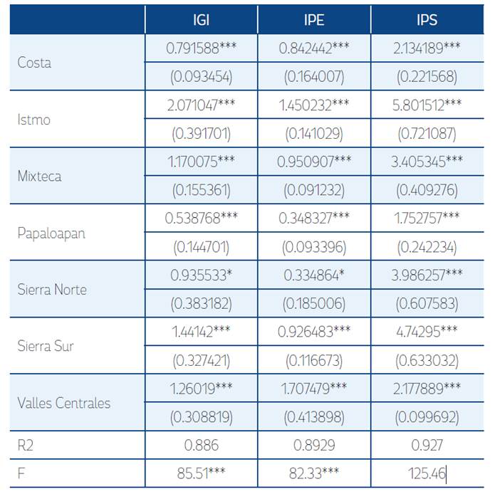
Using the technique of fixed effects by least squares with dichotomous variables (LSDV) we obtained the infrastructure coefficients for each region (Table 13).11 In IPE, the Valles Centrales, Istmo and Mixteca regions have level 1.70, 1.45 and 0.95, respectively, of difference in reference to the Cañada region. In other words, they are the regions that are a bit better in economic infrastructure than the rest of the regions. For the IPS, the Istmo, Sierra Sur and Sierra Norte regions show a level of 5.80, 4.74 and 3.98, respectively, of difference in reference to the Cañada region.
Intermediate regions such as Valles Centrales, Istmo, and to a lesser extent Mixteca, must allocate a greater proportion ofpublic spending to economic infrastructure. The other regions (Cañada, Costa, Papaloapan, Sierra Norte and Sierra Sur) can be classified as lagging, so they require investment in social infrastructure (health and education) to lay the foundations for a more qualified population and create the conditions for them to increase their economic activity in the long term. This does not mean that in the intermediate regions IPS should not be invested and that in the backward regions IPE should not be generated, but in the lagging regions more IPS is invested than is needed.
CONCLUSIONS
Oaxaca’s economic activity is concentrated in two of its eight regions, Valles Centrales and Istmo. Over the 2003 ─ 2013 period the differences in the standard of living, in terms of GDP per capita, have been reduced between regions, going from 8 to 3.5 times the difference between the best and worst positioned regions. In terms of infrastructure as measured by the indices, there have been no significant increases in the years of study. On the contrary, in some cases the indices decrease, especially if the infrastructure indices per inhabitant are considered.
In the research it was possible to verify statistically the impact of physical infrastructure, both social and economic, on the GDP per capita growth of the regions of the state of Oaxaca for the period 2003-2013. The results show that a change in a one unit of the physical social infrastructure positively impacts 1.19% (in the case of infrastructure per km2) or 2.46% (infrastructure per inhabitant) in the regional economic growth.
In the same line, it is proposed that the most dynamic regions (Valles Centrales and Istmo) invest a greater proportion of public spending on economic infrastructure. In contrast, the backward regions must invest in social infrastructure. On the other hand, the negative effect of physical economic infrastructure by geographic dimension on economic growth can be explained by three reasons. First, the state has a deficiency in the provision of economic infrastructure; in other words, the demand for infrastructure of this type exceeds the supply and generates a congestion effect. This occurs in the municipalities with the greatest economic dynamics located in the Valles Centrales and Istmo regions. The second reason is the remarkable geographical dispersion (Oaxaca is the state with the largest number of municipalities, 570, to give an example). This factor means that there is low (or no) infrastructure coverage. Finally, the very rugged topography of the state raises the investment costs and, therefore, little infrastructure is created.
The lack of appropriate regional public policies has meant that the investment made in infrastructure does not generate the expected economic impacts given that the investment policies are prepared based on general conditions and not the particular ones. That is, they do not take local conditions and problems into account. Therefore, it is proposed that regional plans be generated that emphasize the needs of each region.

